Project 2: Fun with Filters and Frequencies!

Part 1.1

Here is my implementation of convolution. I used used numpy functions to handle the actual convolution operations, making it so I only need 2 for loops. Because of this, the runtime is just the size of the image, though I don't know the exact runtime of the list slicing and numpy operations so it is definitely reasonably slower.

1def convolve(image, kernel):
2    img_height, img_width = image.shape
3    kernel_height, kernel_width = kernel.shape
4    
5    pad_height = kernel_height // 2
6    pad_width = kernel_width // 2
7    
8    flipped_kernel = np.flip(np.flip(kernel, axis=0), axis=1)
9    
10    output = np.zeros((img_height, img_width))
11    
12    for i in range(img_height):
13        for j in range(img_width):
14            start_row = i - pad_height
15            end_row = start_row + kernel_height
16            start_col = j - pad_width
17            end_col = start_col + kernel_width
18            
19            region = np.zeros((kernel_height, kernel_width))
20            img_start_row = max(0, start_row)
21            img_end_row = min(img_height, end_row)
22            img_start_col = max(0, start_col)
23            img_end_col = min(img_width, end_col)
24            
25            region_start_row = img_start_row - start_row
26            region_end_row = region_start_row + (img_end_row - img_start_row)
27            region_start_col = img_start_col - start_col
28            region_end_col = region_start_col + (img_end_col - img_start_col)
29            
30            region[region_start_row:region_end_row, region_start_col:region_end_col] = image[img_start_row:img_end_row, img_start_col:img_end_col]
31            
32            output[i, j] = np.sum(region * flipped_kernel)
33    
34    return output

Here is me after applying the box filter. Since the image I took is fairly high resolution, it is hard to tell that it is blurred from the 9x9 box filter, so I included a result on the right that uses an 18x18 box filter.

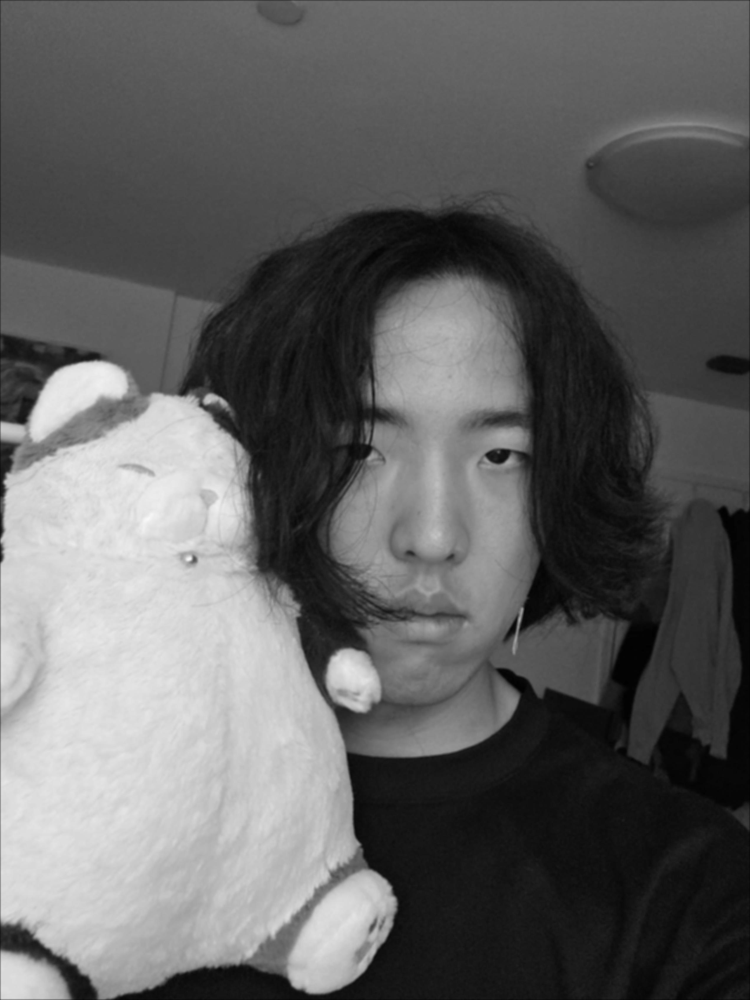
Here is me after applying the 9x9 box filter.

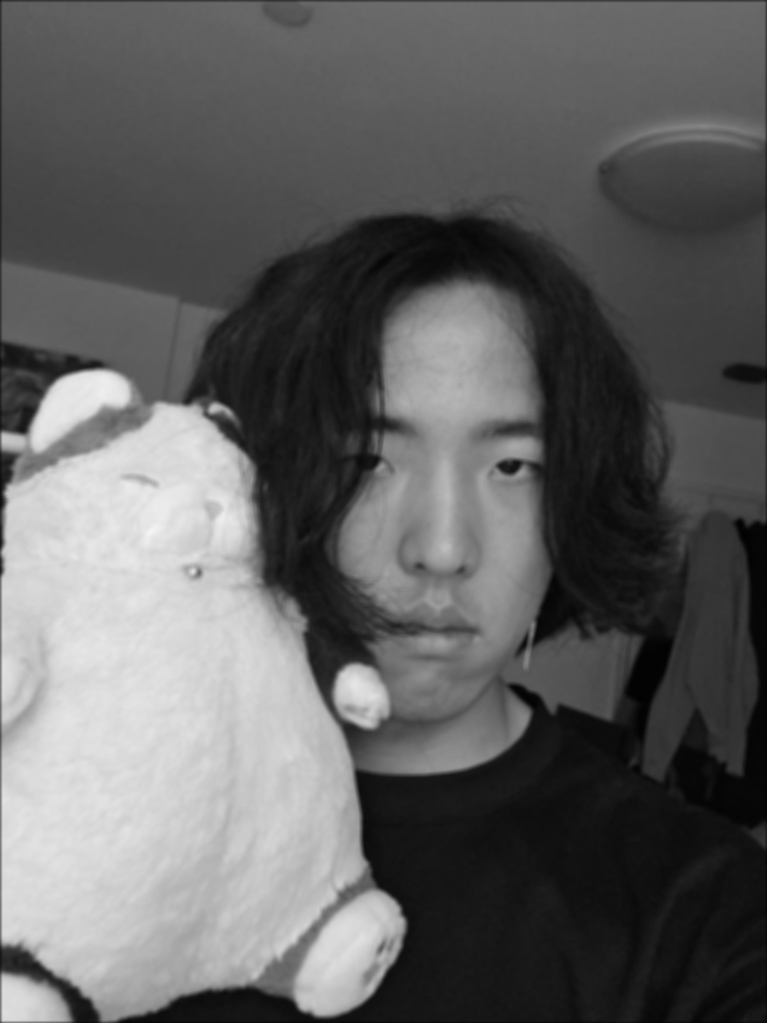
Here is me after applying the 18x18 box filter.

Here is the code for the rest of 1.1 and the finite difference operators. Here are the differences compared to the scipy convolve:
Box filter: 5.968558980384842e-13
Dx operator: 0.0
Dy operator: 0.0

1def q1_1():
2    img = Image.open('q1.jpg').convert('L')
3    image = np.array(img, dtype=np.float64)
4    
5    box_filter = np.ones((9, 9)) / (9 * 9)
6    box_filtered = convolve(image, box_filter)
7    
8    Dx = np.array([[1, 0, -1]])
9    Dy = np.array([[1], [0], [-1]])
10    
11    dx_result = convolve(image, Dx)
12    dy_result = convolve(image, Dy)
13    
14    scipy_box = signal.convolve2d(image, box_filter, mode='same', boundary='fill', fillvalue=0)
15    scipy_dx = signal.convolve2d(image, Dx, mode='same', boundary='fill', fillvalue=0)
16    scipy_dy = signal.convolve2d(image, Dy, mode='same', boundary='fill', fillvalue=0)
17    
18    
19    print("Max differences from scipy:")
20    print(f"Box filter: {np.max(np.abs(box_filtered - scipy_box))}")
21    print(f"Dx operator: {np.max(np.abs(dx_result - scipy_dx))}")
22    print(f"Dy operator: {np.max(np.abs(dy_result - scipy_dy))}")
23    
24    Image.fromarray(np.clip(box_filtered, 0, 255).astype(np.uint8)).save('out/q1_box_filtered.jpg')
25    Image.fromarray(np.clip(np.abs(dx_result), 0, 255).astype(np.uint8)).save('out/q1_dx_result.jpg')
26    Image.fromarray(np.clip(np.abs(dy_result), 0, 255).astype(np.uint8)).save('out/q1_dy_result.jpg')

Here is the picture convolved with the finite difference operators. You may need to zoom in to see the lines since they are very fine.

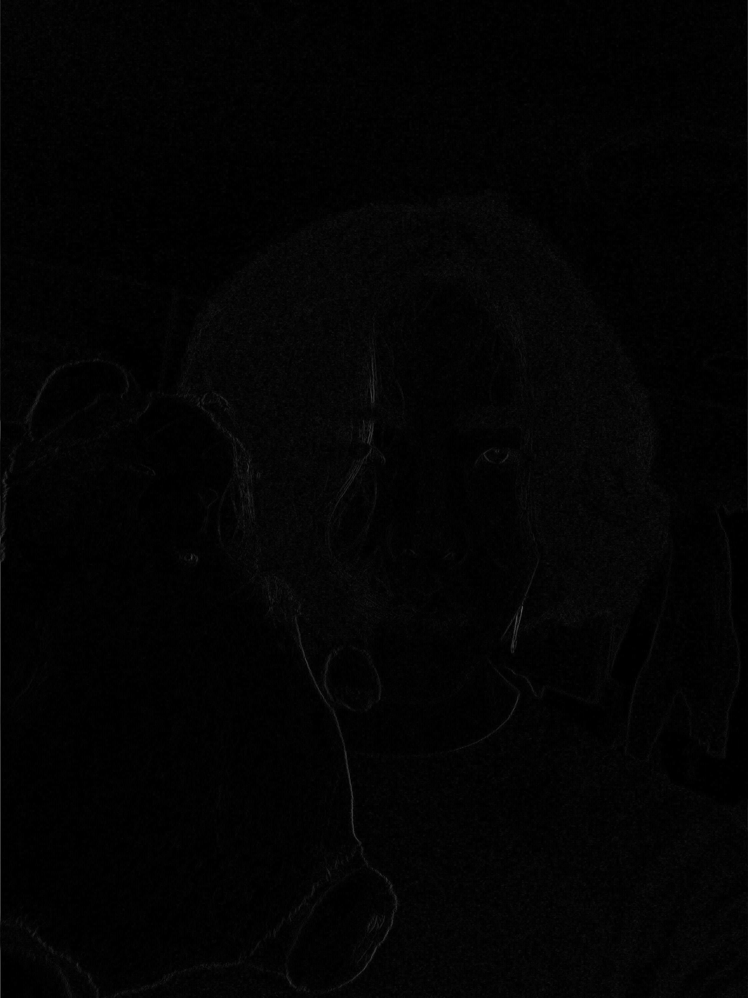
Here is the picture convolved with the Dx operator.

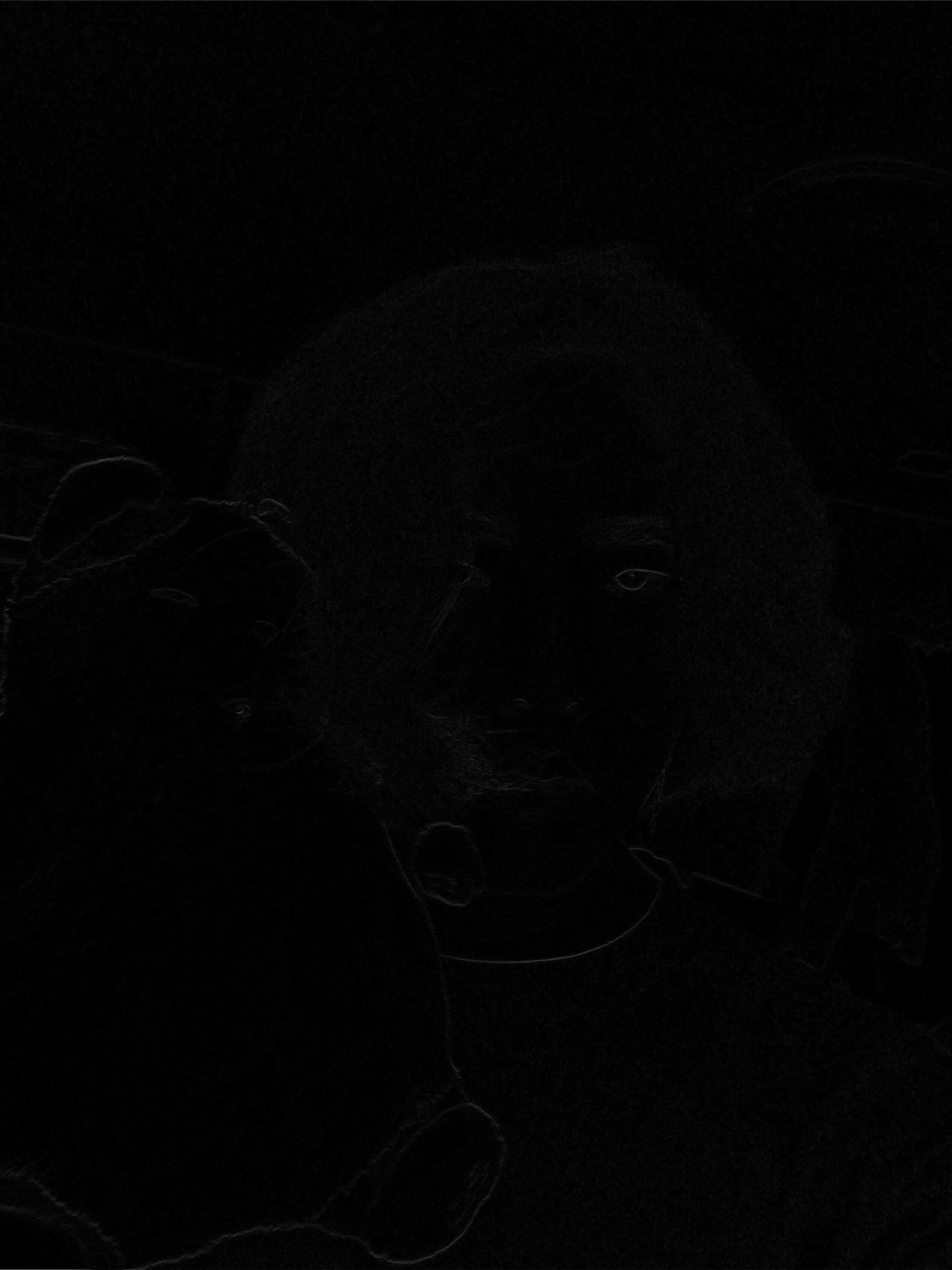
Here is the picture convolved with the Dy operator.

Part 1.2

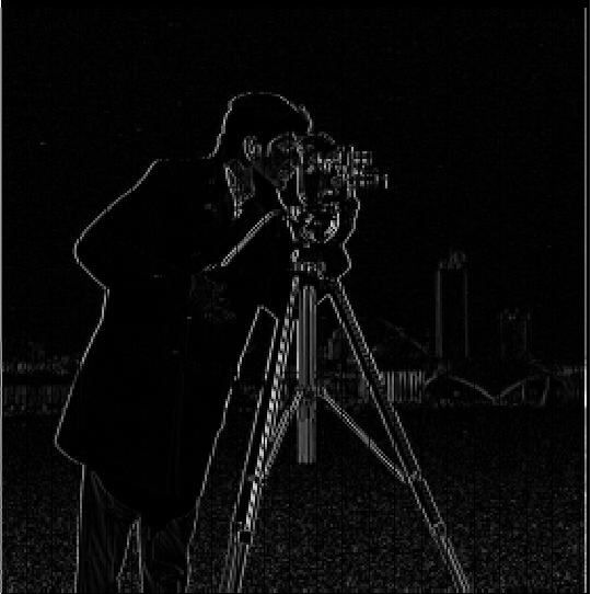
Here is the picture convolved with the Dx operator.

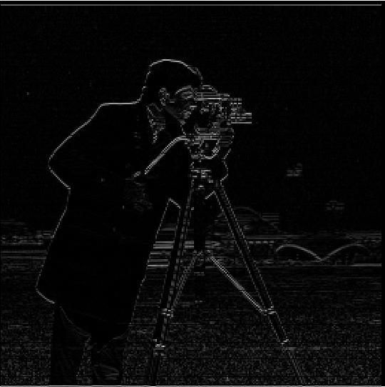
Here is the picture convolved with the Dy operator.

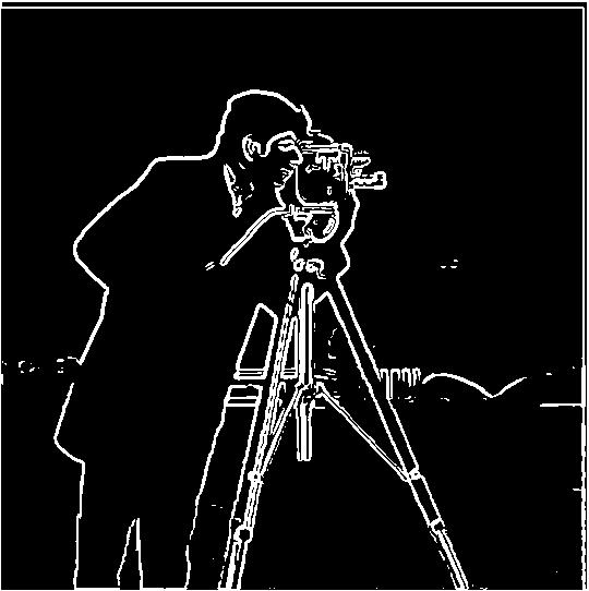
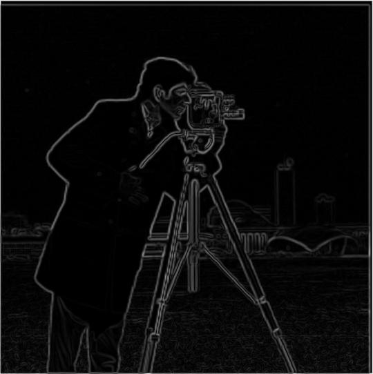
Above are the results of the finite difference operators. Below are the results of gradient magnitude and edge images. For the edge image, choosing a lower threshold would result in more noise coming in from the grass at the bottom, and choosing a higher threshold would result in less noise from the grass but also not show some of the buildings in the background. Ultimately, I opted for a slightly higher threshold since I think the background buildings aren't as important and the grass noise is very annoying.

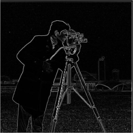
Here is the gradient magnitude.

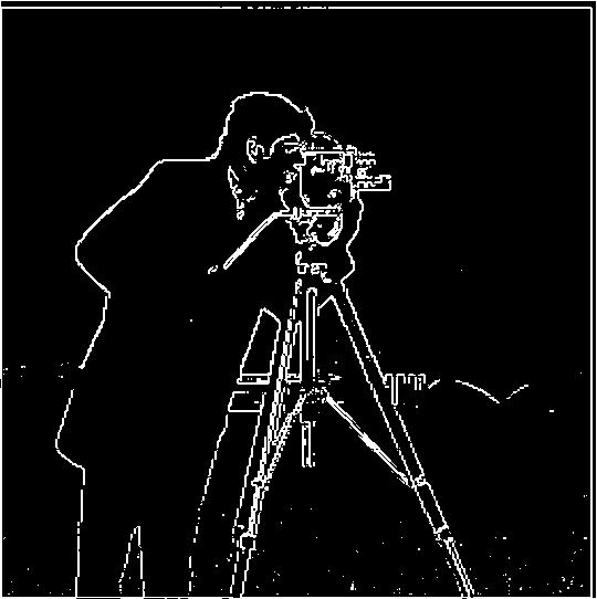
Here is the edge image.

Part 1.3

Here are the results of edge detection on the blurred image and the single convolution image. They appear to be the exact same, which is good.

Here is the edge image on the blurred image.

Here is the edge image by first convolving the filters together than convolving the result with the dog image.

The main differences of these images compared to the edge image on the original image is that the lines are a lot smoother and more well defined, especially in noisy areas like near the bottom. It is still hard to capture the buildings in the background without capturing too much noise from the grass in the foreground, but that would probably require more sophisticated denoising techniques. Below are the gradient magnitude images for both the blurred and single convolution images.

Here is the gradient magnitude on the blurred image.

Here is the gradient magnitude on the single convolution image.

Part 2.1

Here are the results of the sharpened Taj Mahal images. Since it is kind of hard to tell the sharpened effect from alpha = 1.0, I also included the version with double the sharpening on the right.

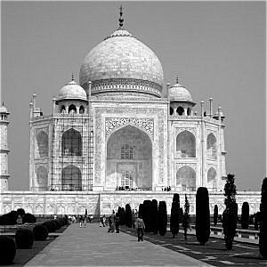
Here is a sharpened image with alpha 1.0 (adds 1x the high frequencies)

Here is a sharpened image with alpha 2.0 (adds 2x the high frequencies)

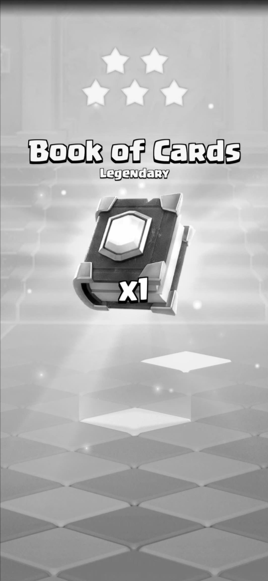
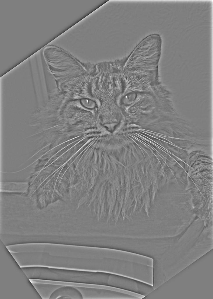
The way sharpening works is that we first blur the image with a gaussian blur, which acts as a low pass filter. Then, we subtract the blurred image from the original image, which acts as a high pass filter. Since the higher frequencies often contain the details and perceived "sharpness" of an image, we can just add back the high frequencies to the original image to get a "sharper" version of the image. However, this obviously means the new image isn't the really the same, as we are adding more information to the image. When too much sharpness is added, it also appears kind of deep fried. Here is an example of the a sharpened image of the legendary book of cards I got from a 5 star lucky drop in Clash Royale.

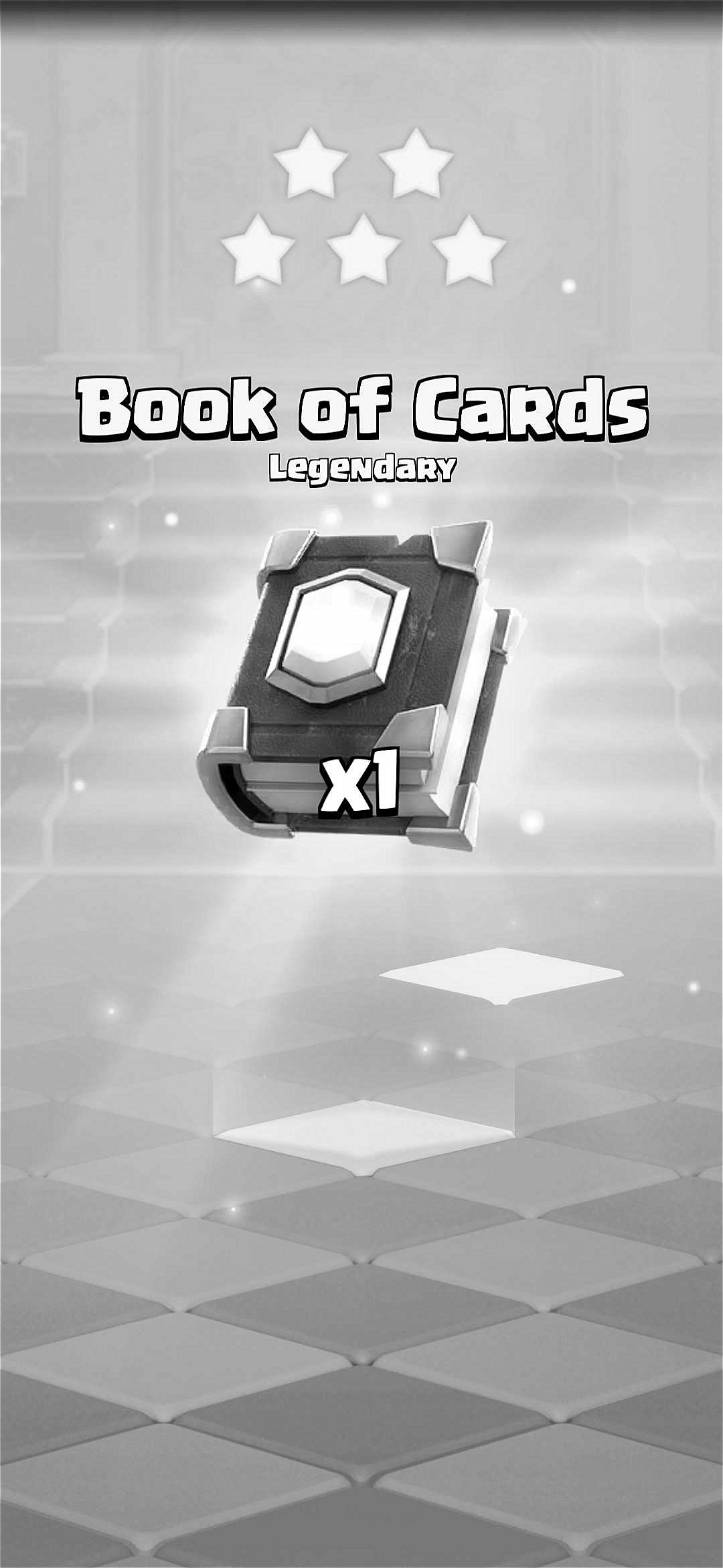
Here is the image with alpha 1.0

Here is the sharpened image with alpha 10.0 to really show the effect (it is harder to see since the image is so high resolution compared to the Taj Mahal).

Here is the sharpened version of the blurred image of the book of cards. It is kind of hard to tell a difference since the image itself is mainly higher frequencies, meaning the sharpening applies to most of the image and the blurring doesn't really do much. I even blurred the original image twice to make it more blurry before sharpening and you can tell in the alpha=1.0 version, but in the alpha=10.0 version it looks very similar to the sharpened non blurred image.

Here is the sharpened blurred image with alpha 1.0

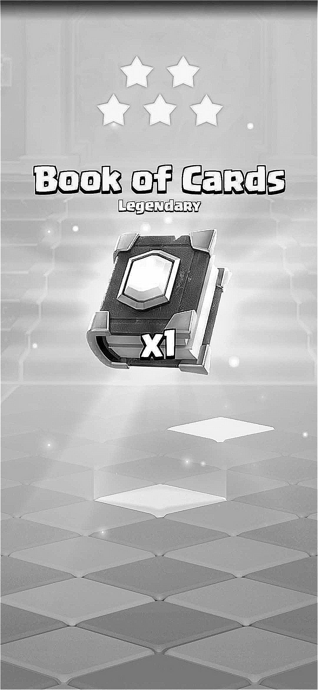
Here is the sharpened blurred image with alpha 10.0

Part 2.2

Here is the hybrid image I generated of Derek and Nutmeg. The borders of the Nutmeg image can be see due to the alignment, but I didn't crop it and just used the borders of the original Derek image as the size of the hybrid image. I had to mess around with the thresholds for the high and low pass filters to get the best results. In this case, if you squint a lot you can't even see Nutmeg at all, so I think it works well.

Derek and Nutmeg

Here is the entire process for generating the Derek and Nutmeg image. First, here are the images after alignment and filtering. For alignment, I used the given alignment function and aligned their eye positions. Below that are the ffts of the images after filtering.

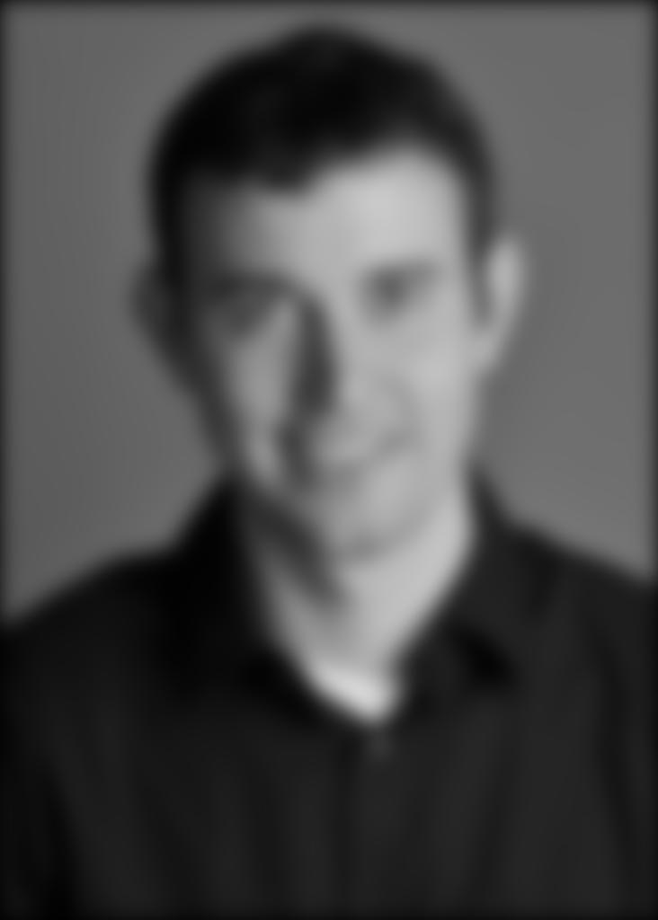
Derek with low pass

Nutmeg aligned with high pass

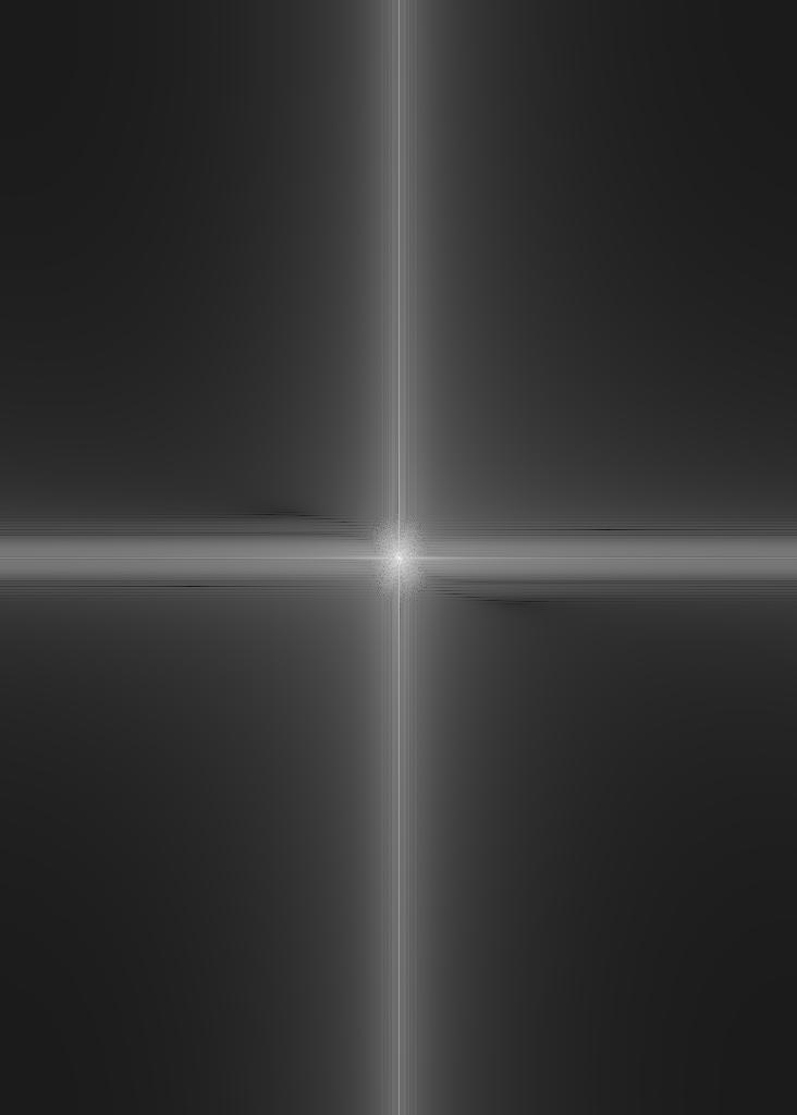
Low Pass FFT

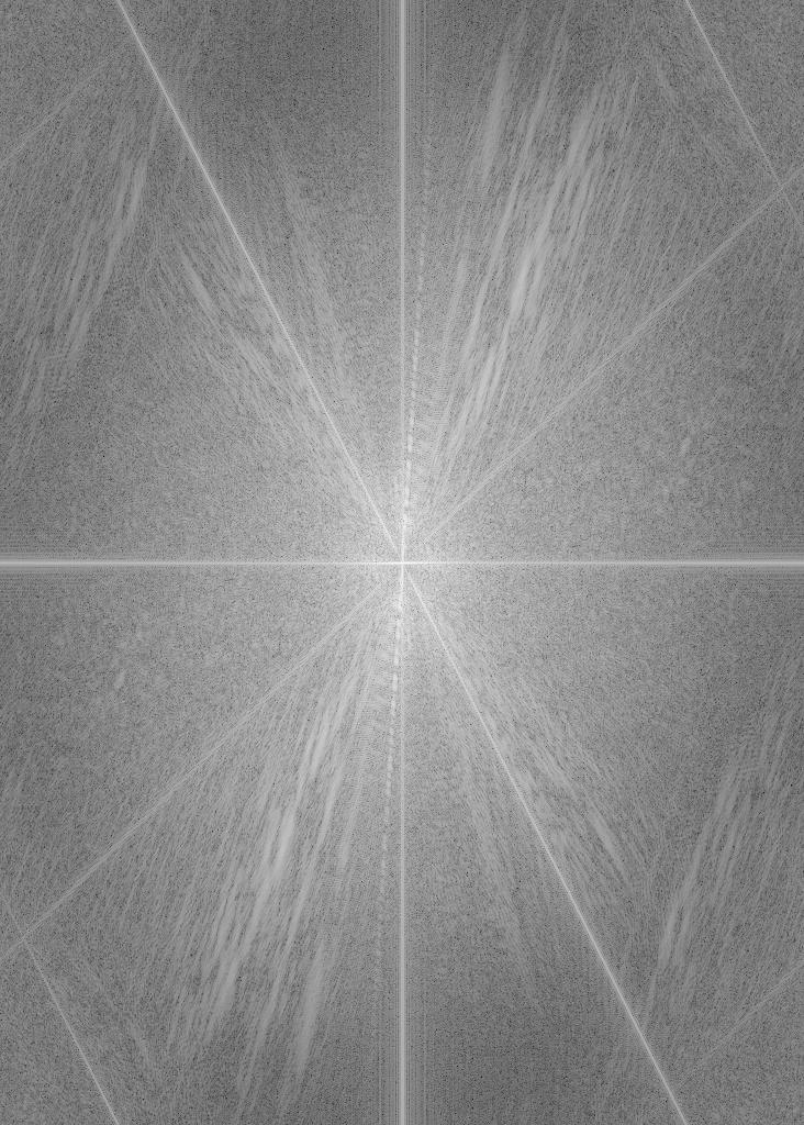
High Pass FFT

With some testing, ended up using sigma = 7.0 for the high pass filter and sigma = 12.0 for the low pass filter. Maybe I'm biased since I was testing it from a close position, but I found that the nutmeg image will usually dominate the hybrid image more so than the derek image, so I ended up using a higher sigma for the low pass filter. Here is the fft of the hybrid image.

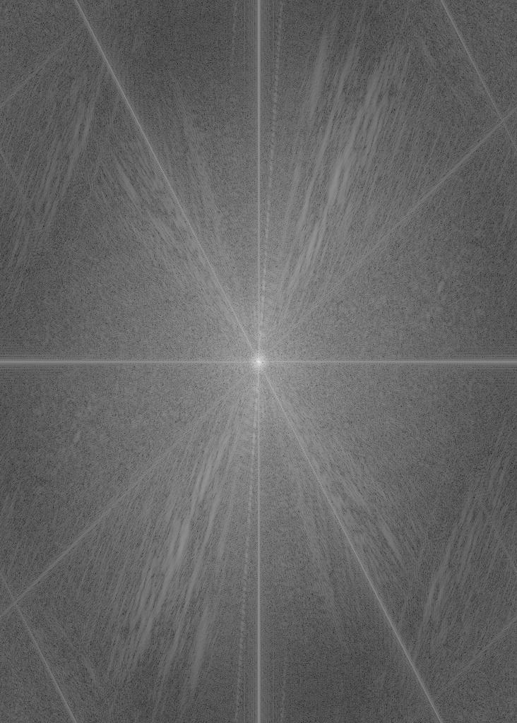
FFT of derek and nutmeg hybrid

Here are some other hybrid images that I made. First, we have a hybrid between a troll face and a suspiciouslly troll face shaped pile of pans. This image of pans was one of a collection of images bearing a resemblance to a troll face, and interestingly it already kind of has that hybrid image effect built in. By putting a low pass version of the troll face on top, it just becomes a lot easier to see.

Troll face

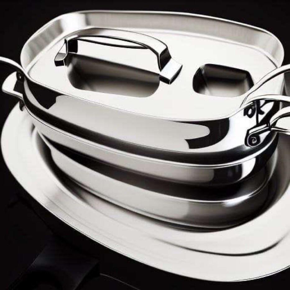
Pans

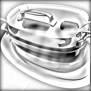
The hybrid image

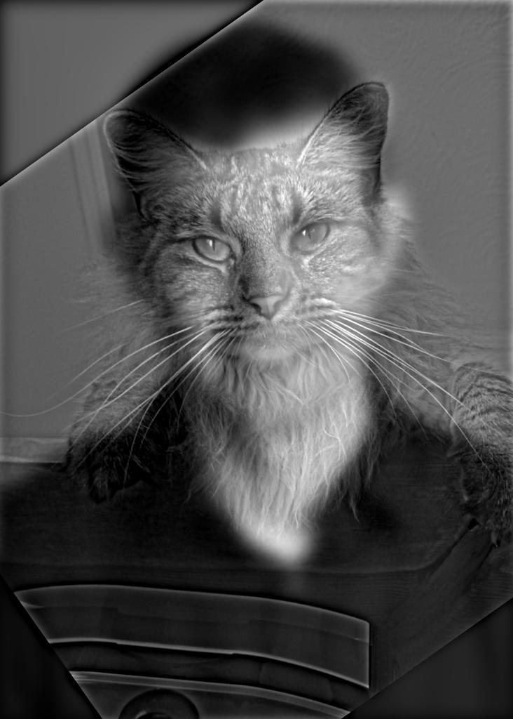
Next, I made a hybrid between my cat and a squirrel. Their shapes didn't really align too well, but if you squint a lot you can see the cat.

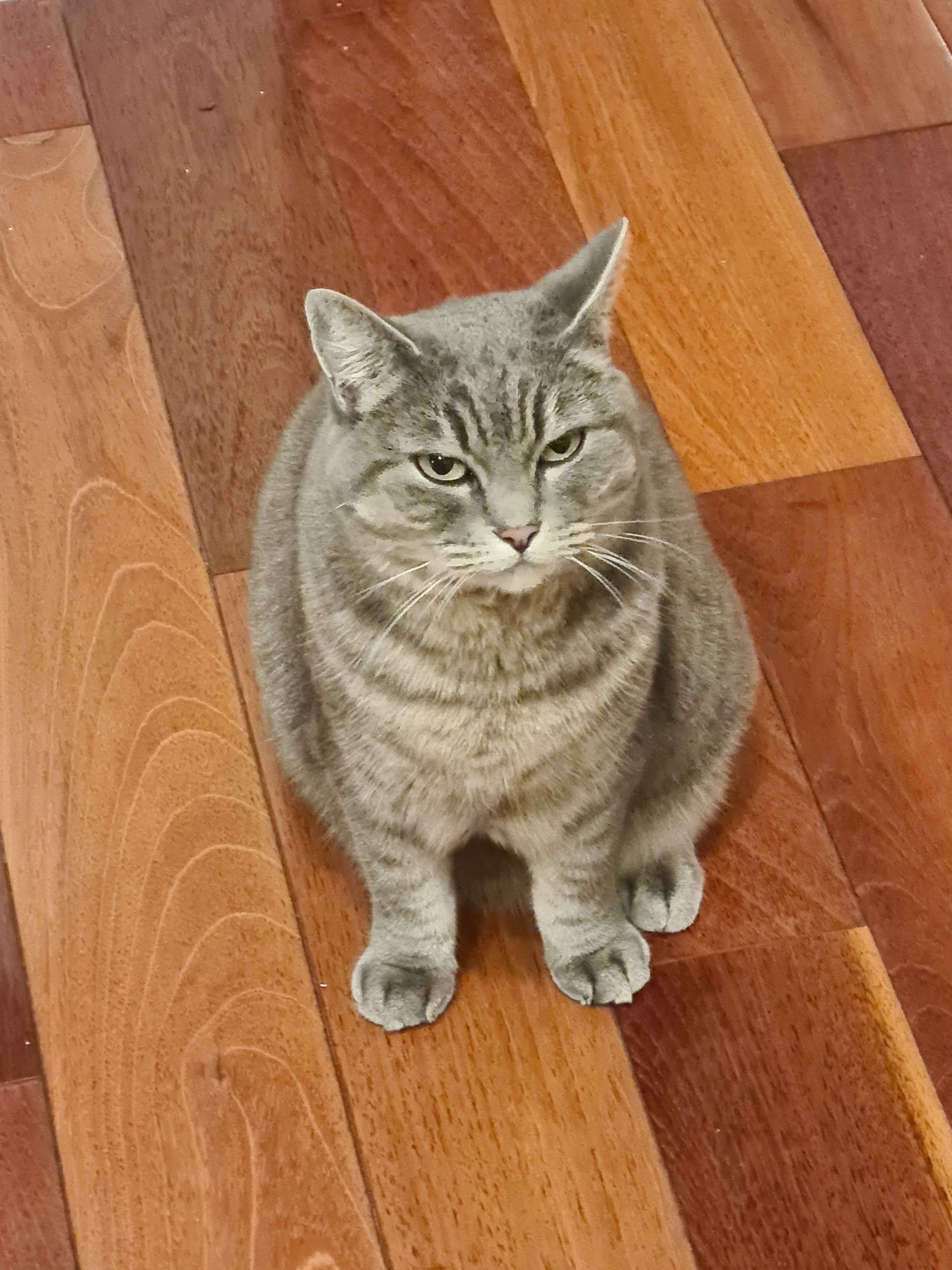
Cat

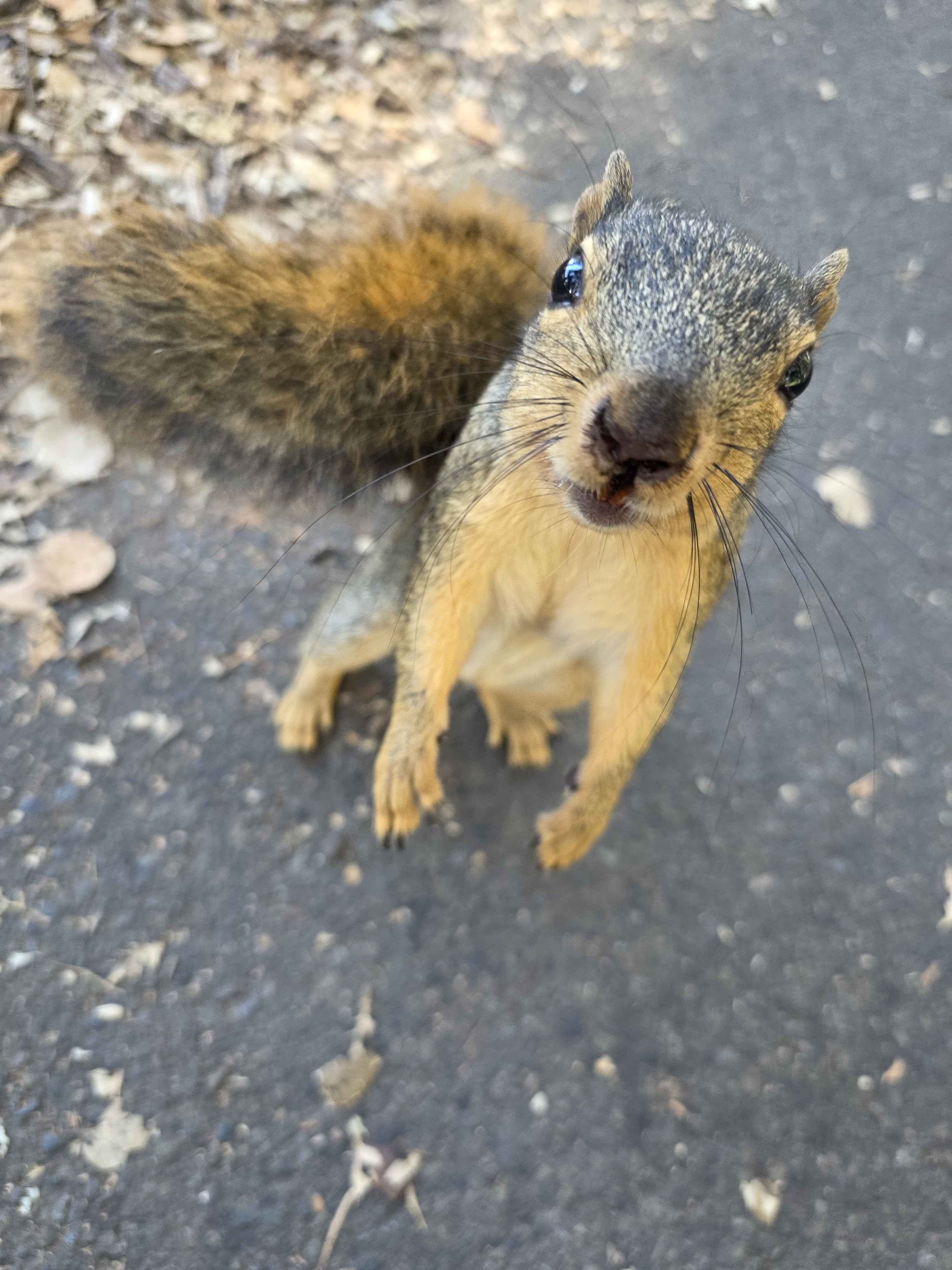
Squirrel

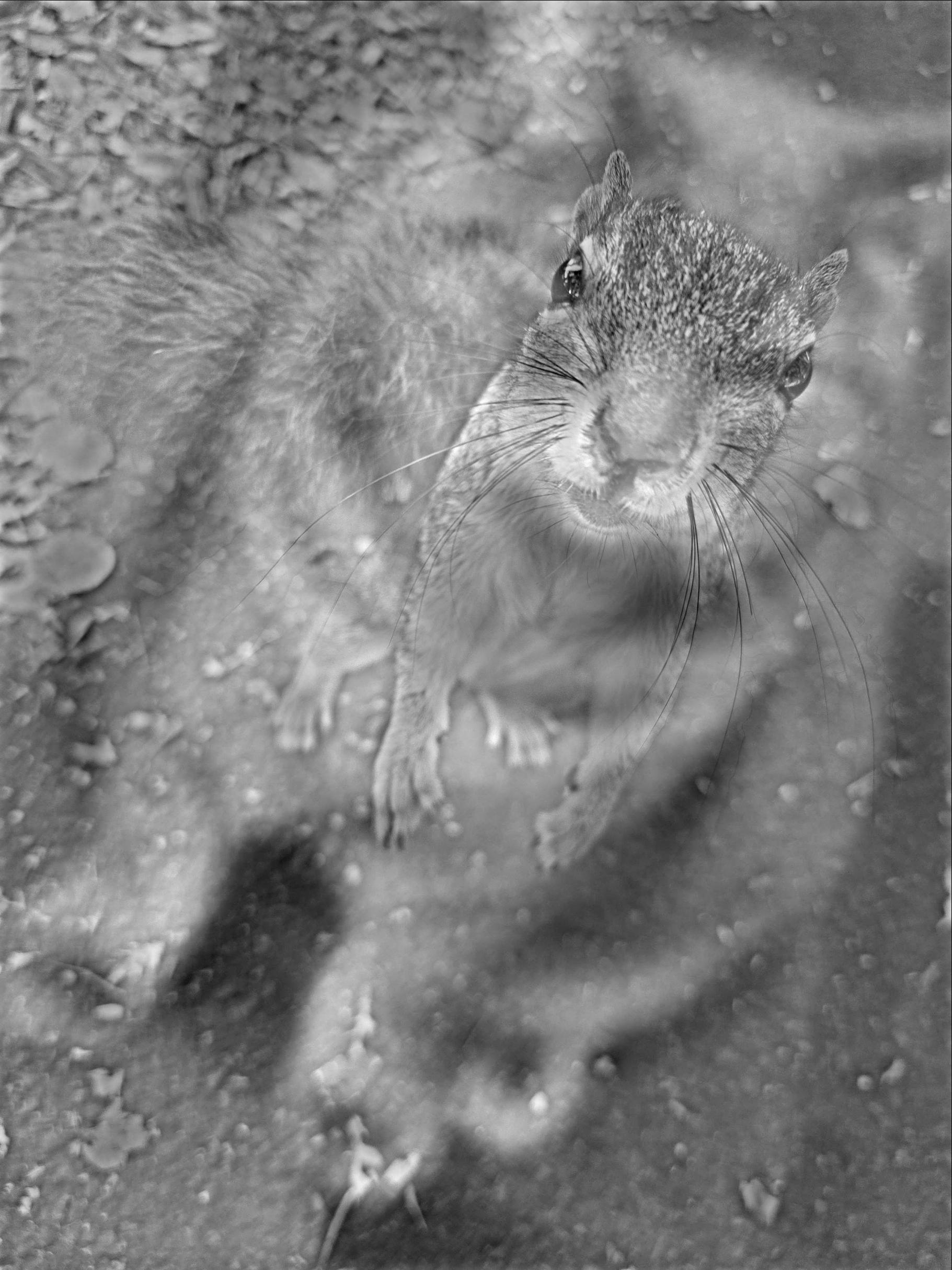
The squirrel cat hybrid

Part 2.3

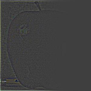
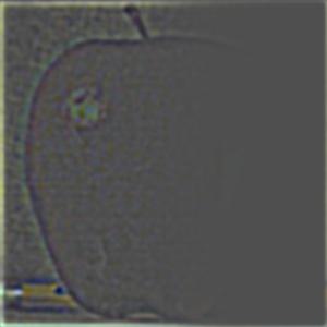
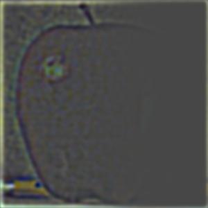
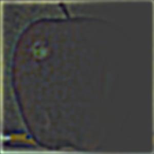
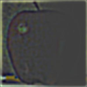
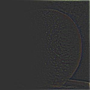
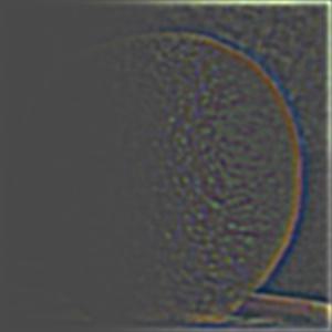
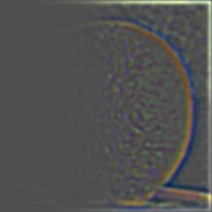
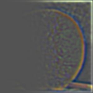
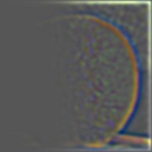
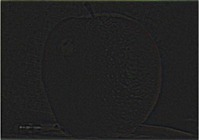
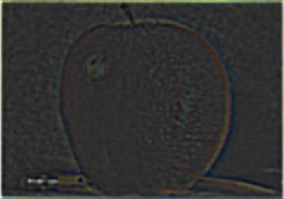
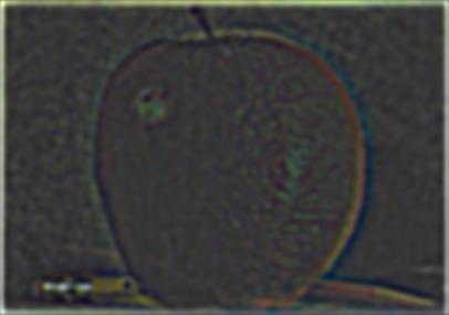
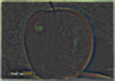
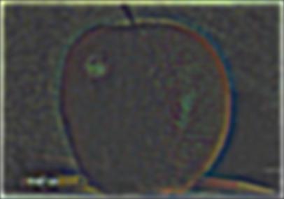
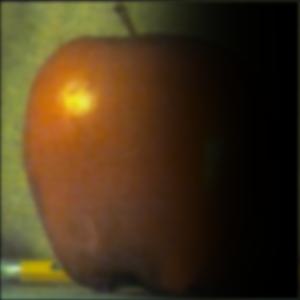
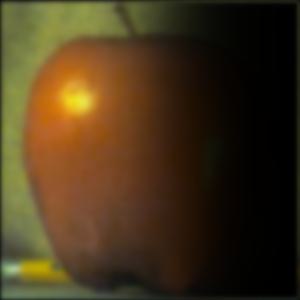
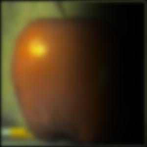
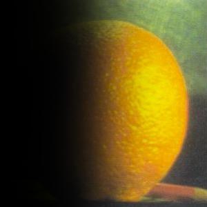
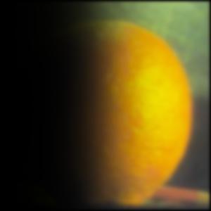
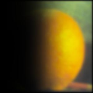
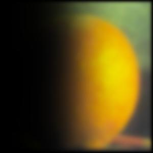
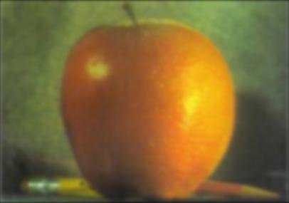
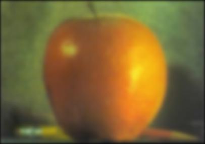
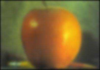
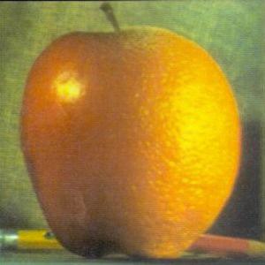
Here are the gaussian and laplacian stacks of the orange, apple, and oraple. I chose to use 6 levels by default, which is what I will use for the hybrid images in 2.4 as well.

Apple Laplacian Stack

Orange Laplacian Stack

Oraple Laplacian Stack

Apple Gaussian Stack

Orange Gaussian Stack

Oraple Gaussian Stack

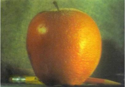
Part 2.4

The oraple

Above is my generated oraple. Below, I created a blend of two cakes from UDessertStory (or whatever that place on shattuck is called). For this one, I made the border fairly solid (so basically the alpha interpolation with a steeper curve), as it made more sense for this image. I did just realize that the cakes are facing different directions, but whatever.

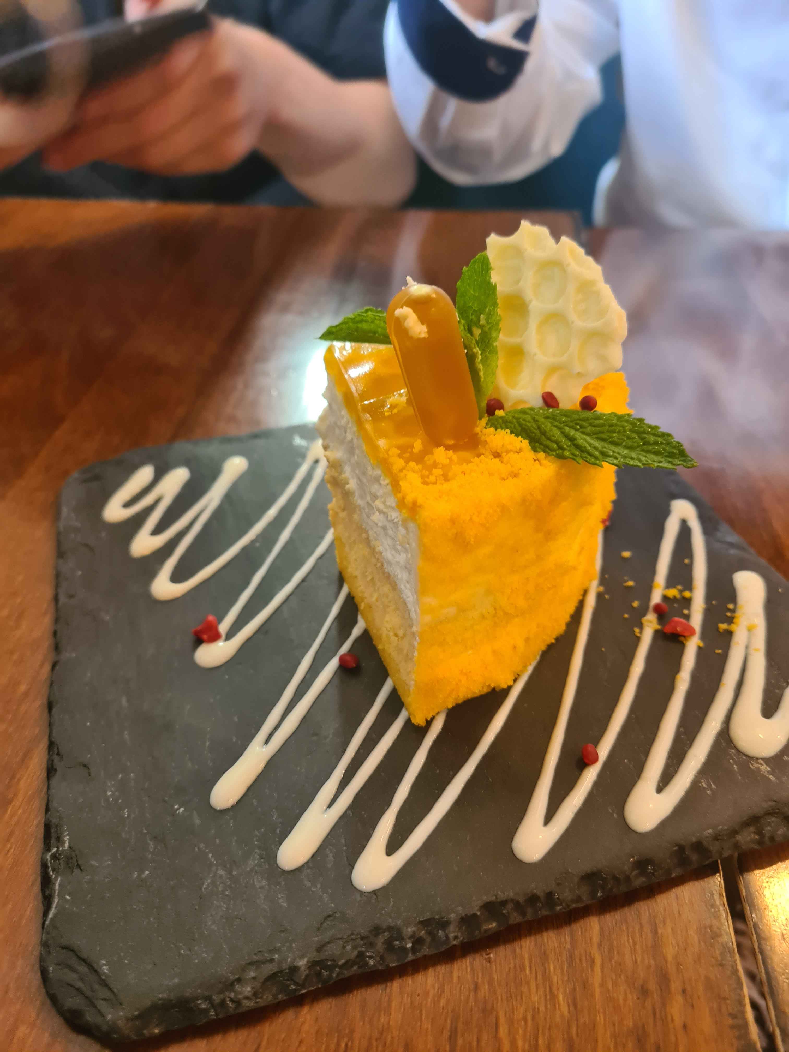
Cake 1

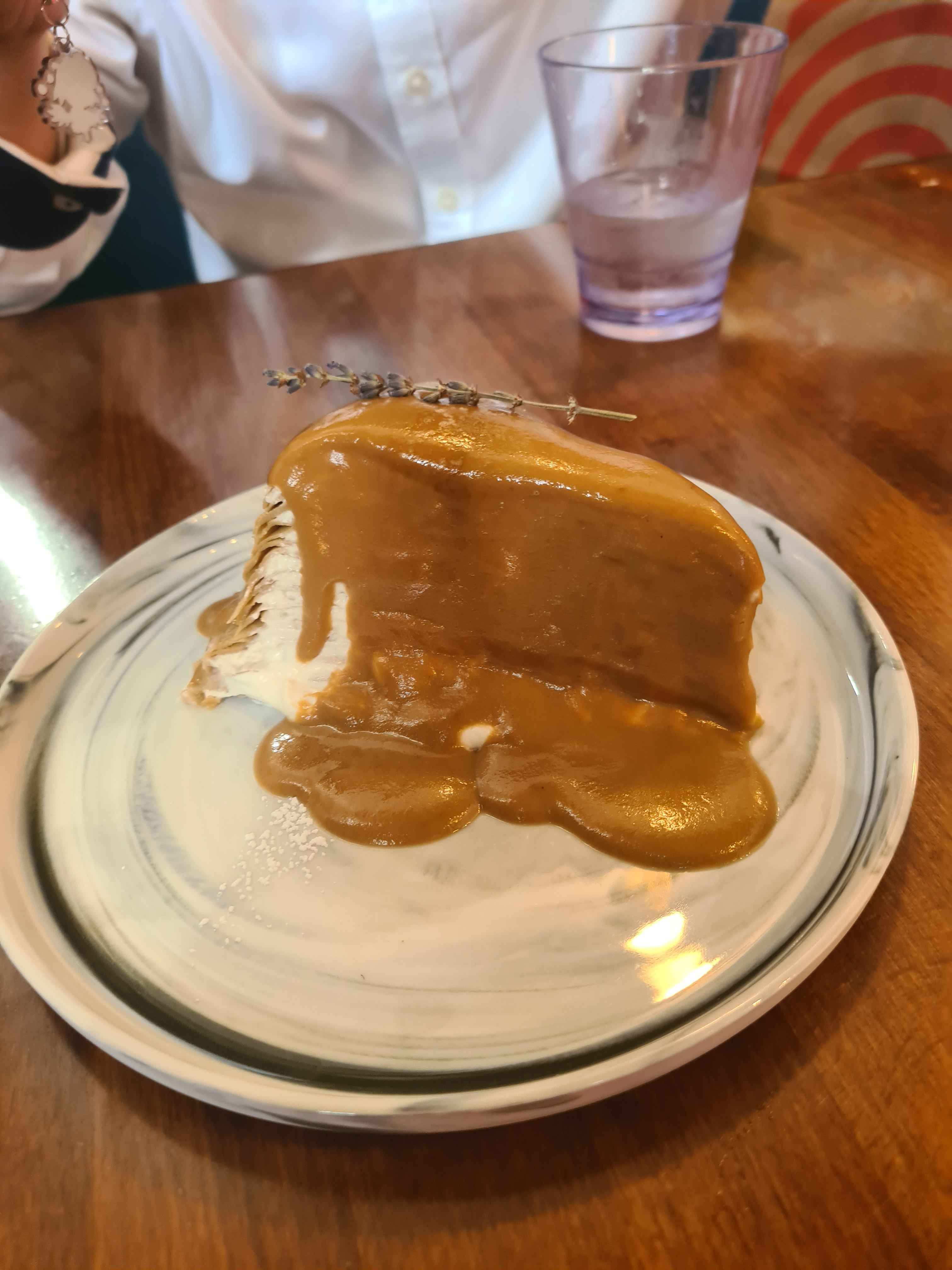
Cake 2

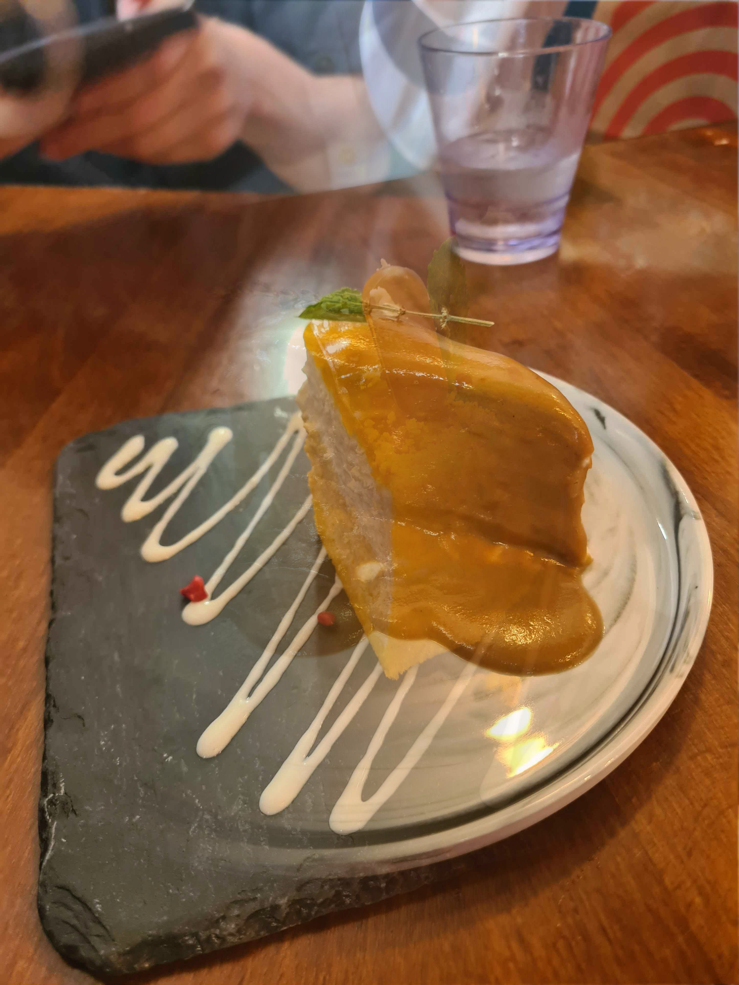
The cake hybrid

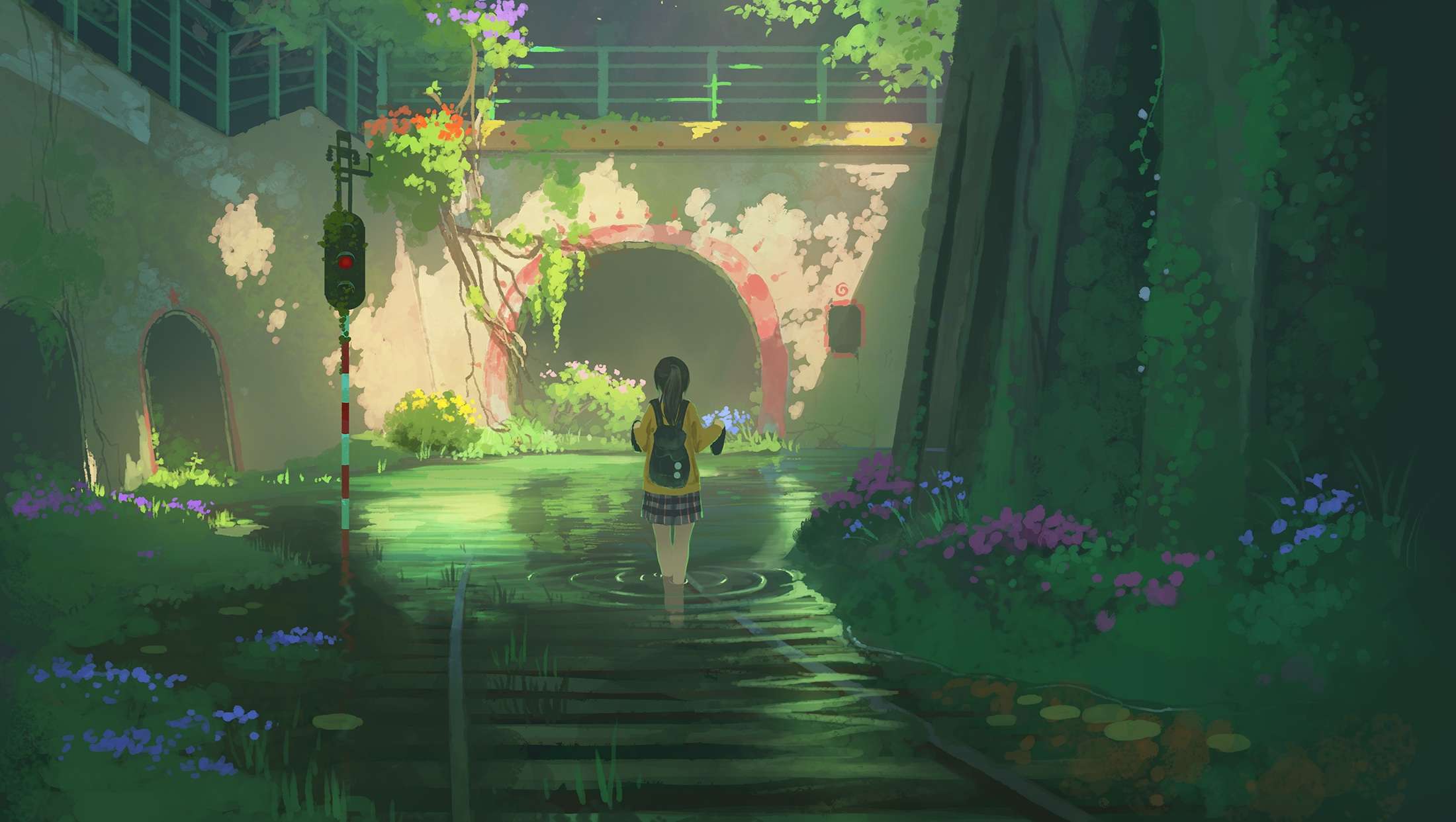
Below, I blended together some artwork from one of my favorite artists, Nauimusuka. Here, I blended them together with the same technique as before, but I had to move the border to the left as well as making it softer to create a better transition. Ultimately, I wanted the girl in the middle of the second picture to still be the main focus on the blended image, so really only the left side of the image looks different compared to the original.

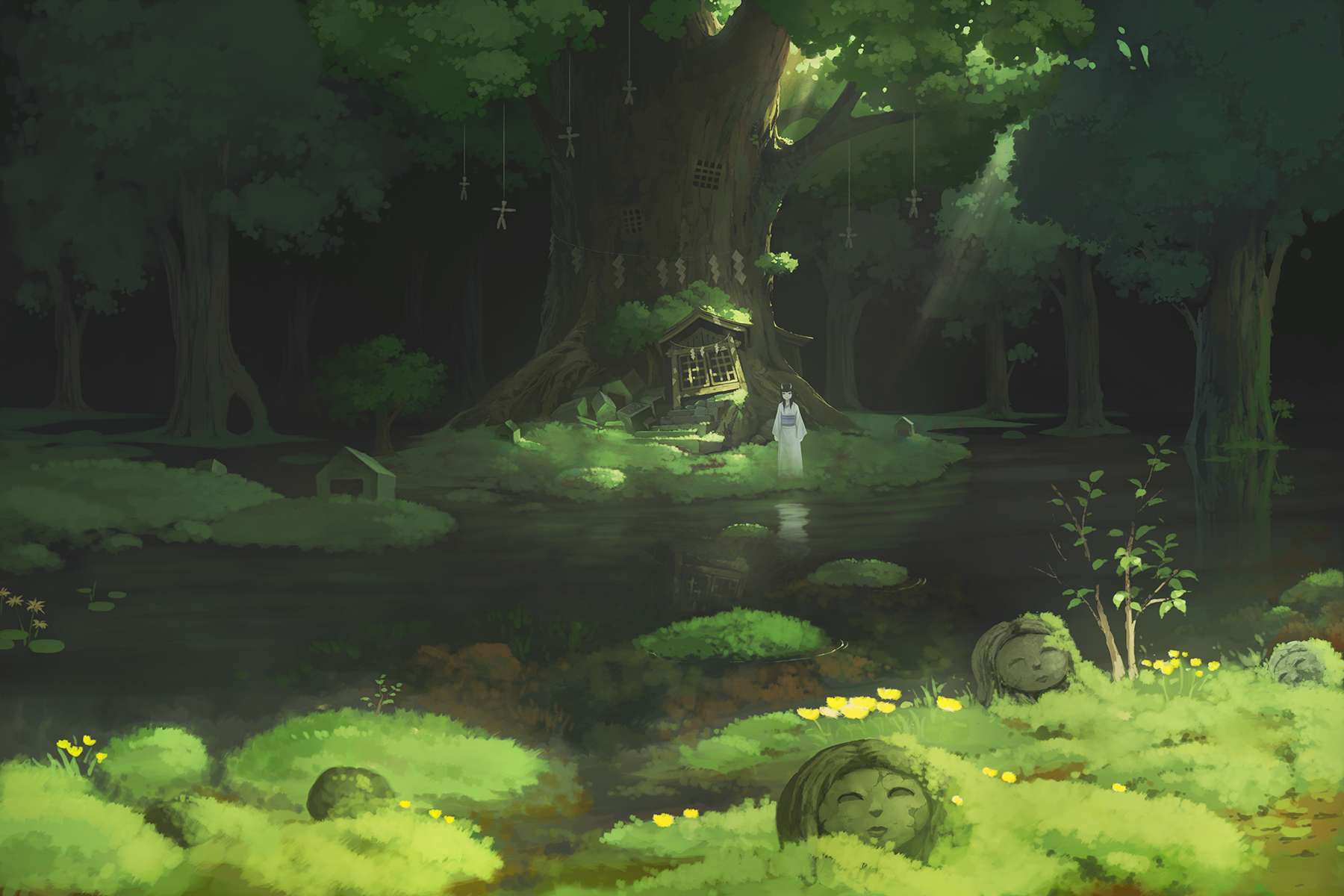
First image (I forgot the names sorry)

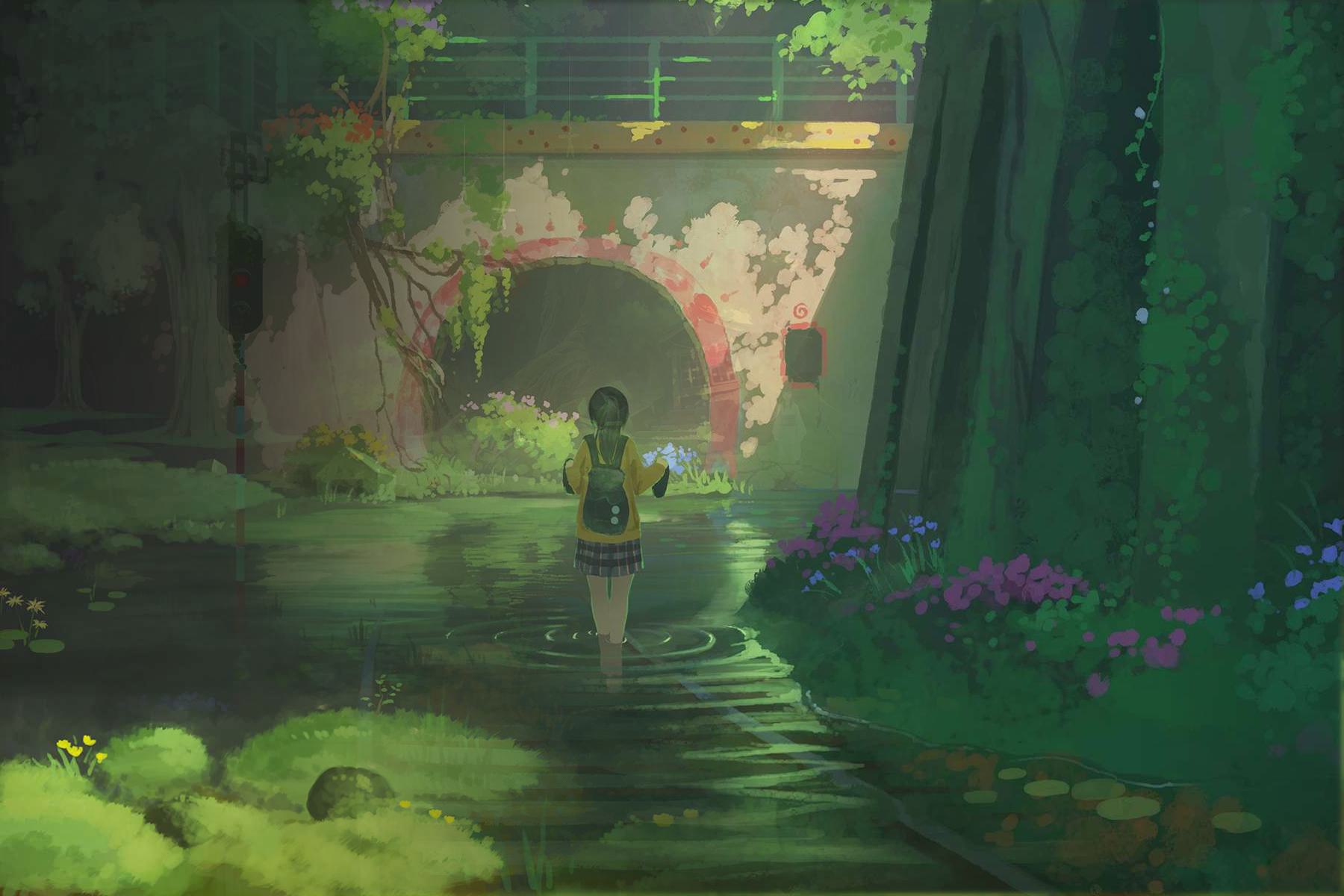
Second image.

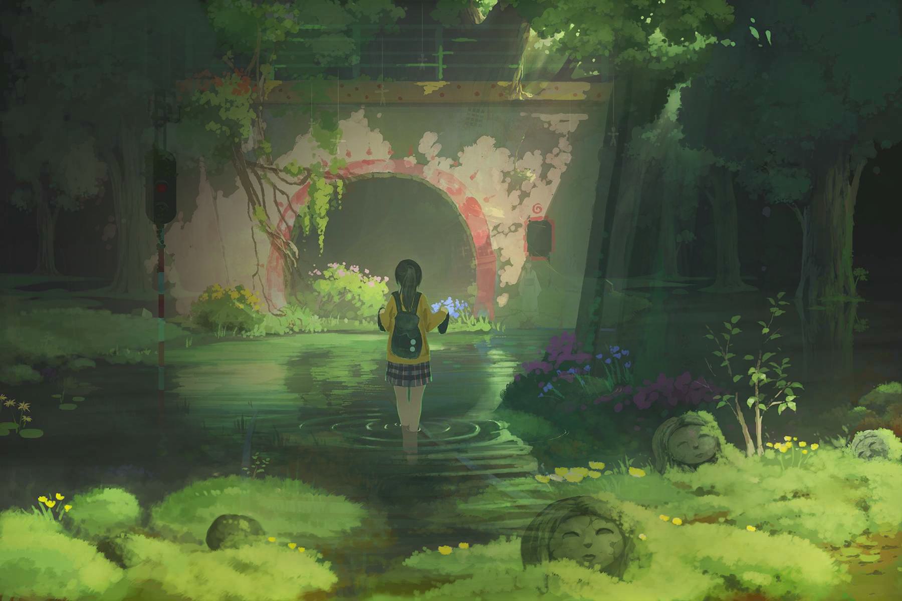
The blended image.

Building on this idea, I wanted to create a custom mask that was a circle in the middle instead of a vertical line. For this, I based the alpha values of both images on the distance from the center of the image, using np.tanh to create the smooth interpolation. This also lets me control the steepness of the interpolation, similarily to before. You can see it really looks like a smooth transition on all sides due to the circle, using the subject from the second image and the background from the first image. Overall, I am very happy with how it turned out.

The final image.