Project 3: [Auto]Stitching Photo Mosaics

Overview

The link is https://aaronx.me/cs180/proj3

Part A.1

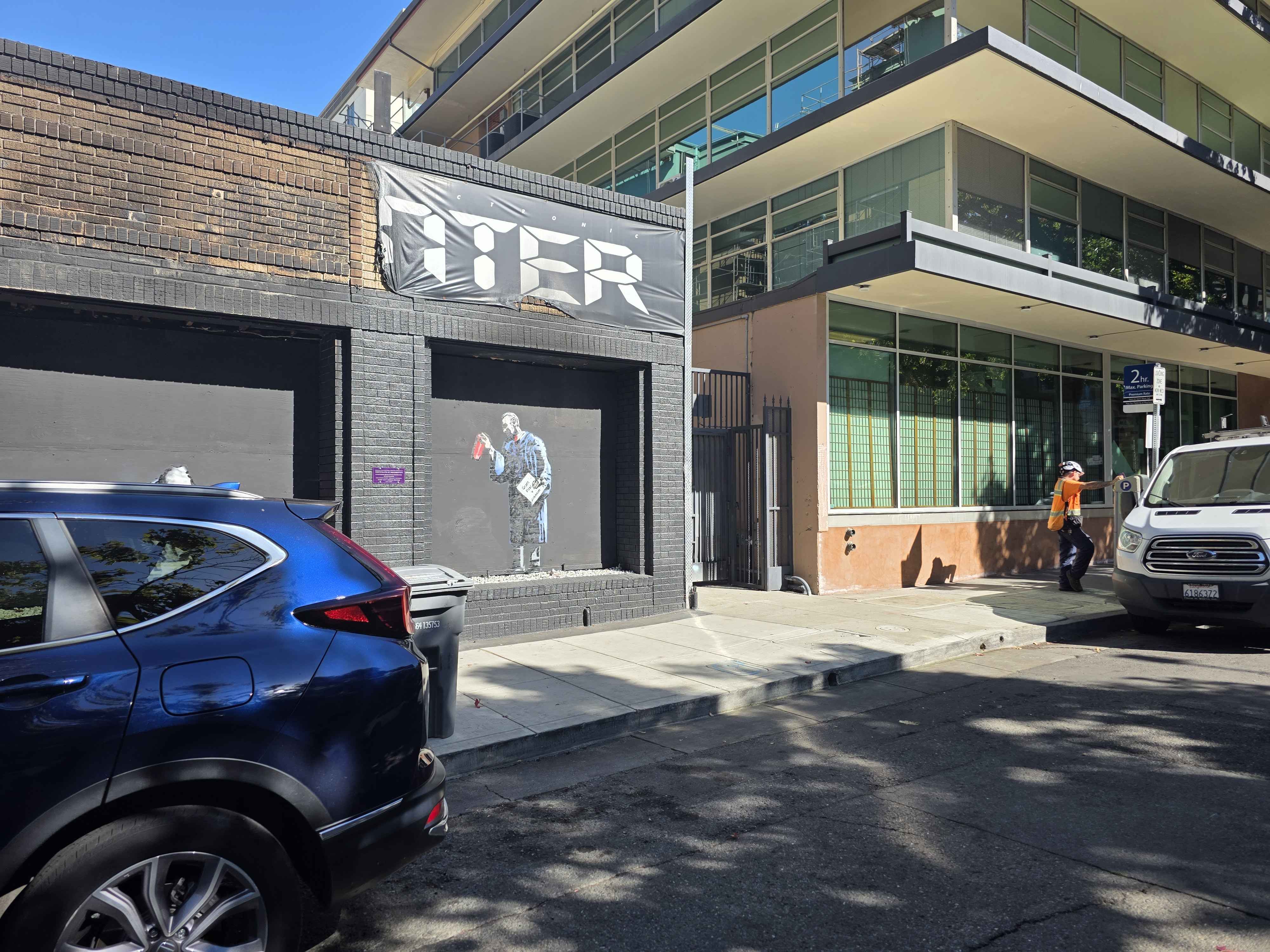
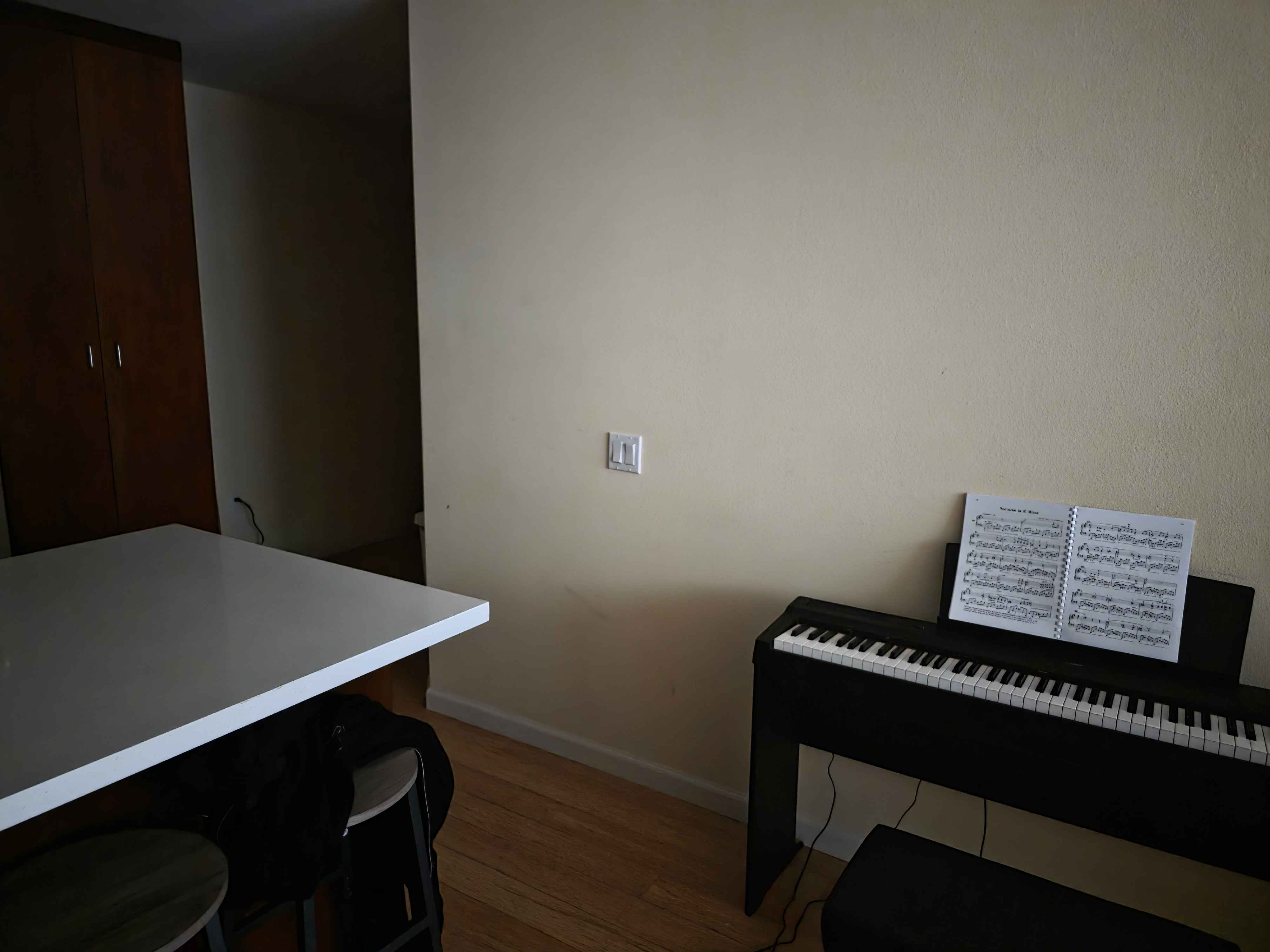
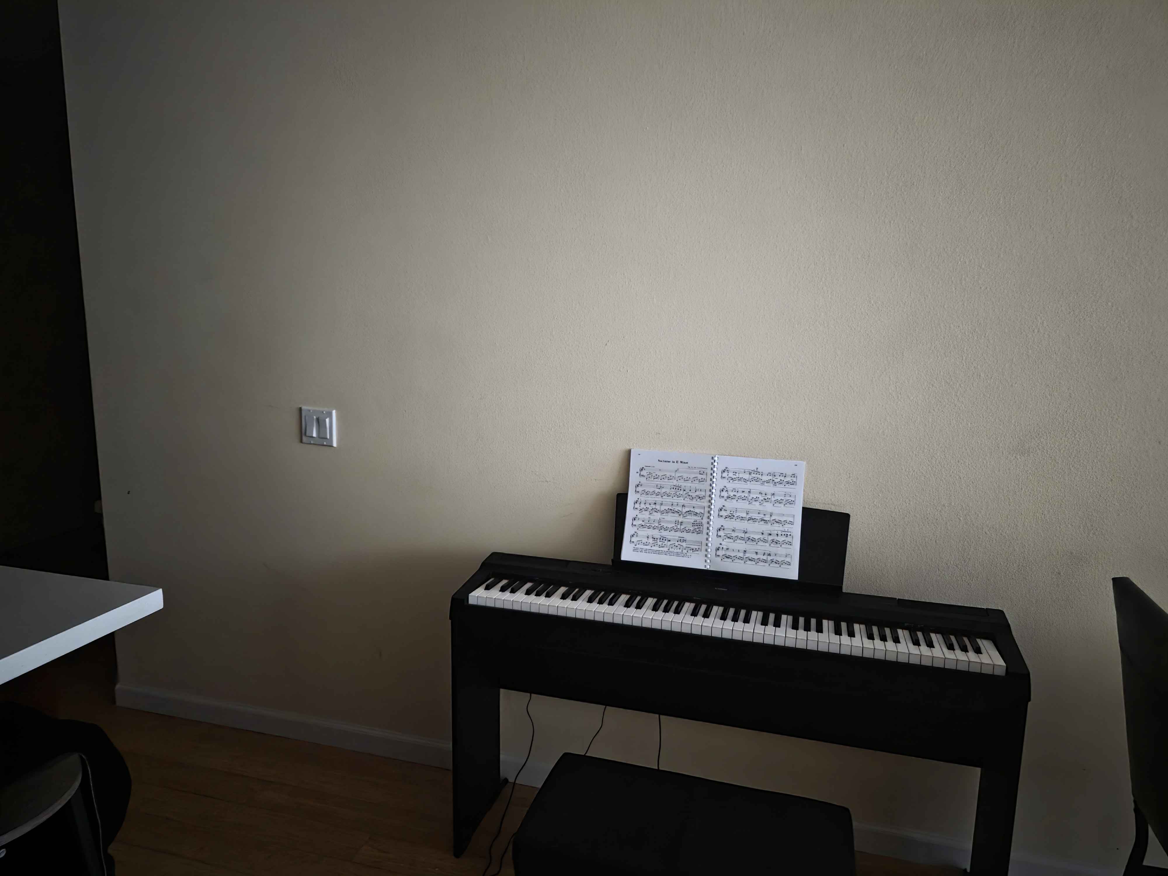
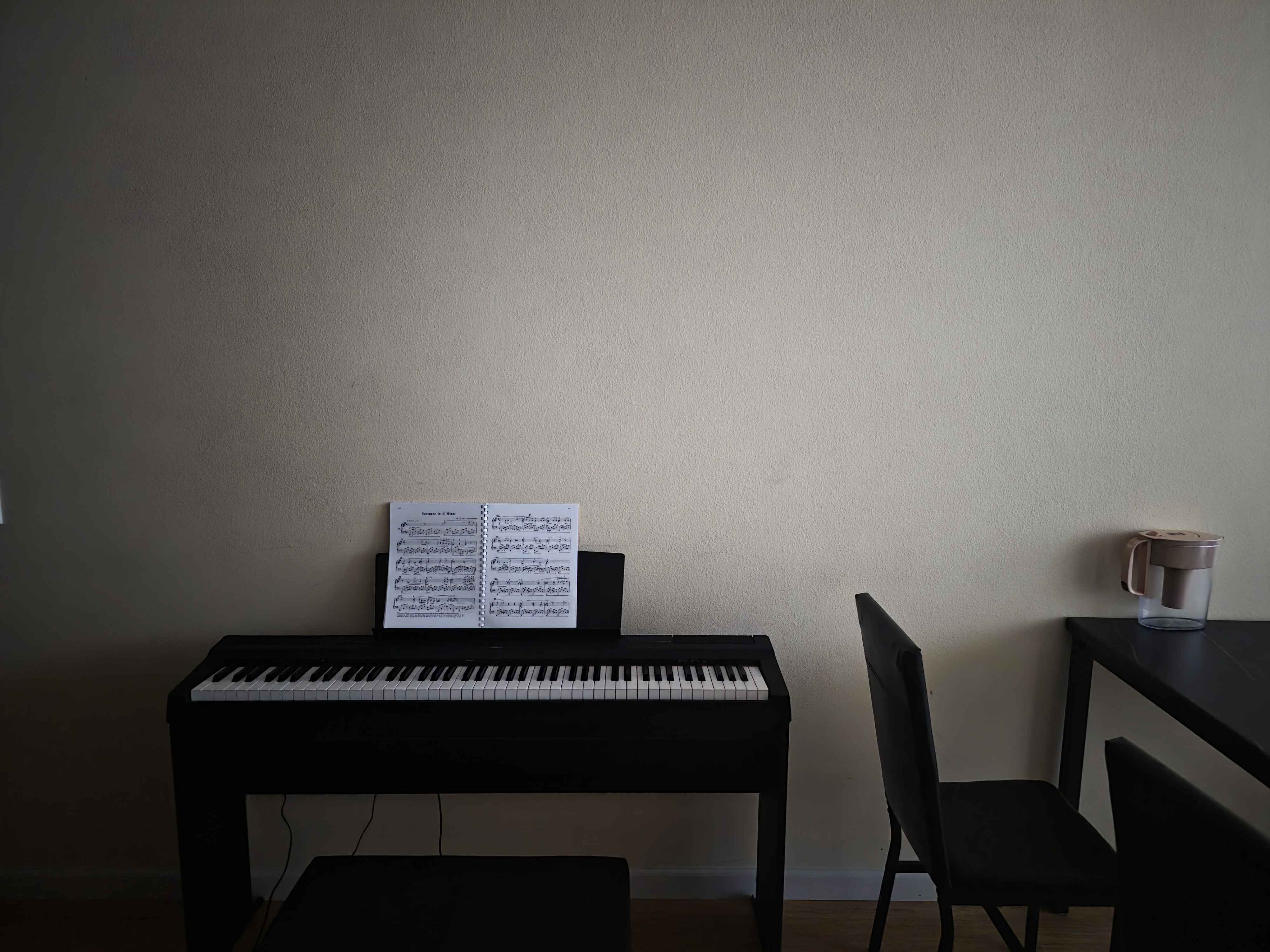
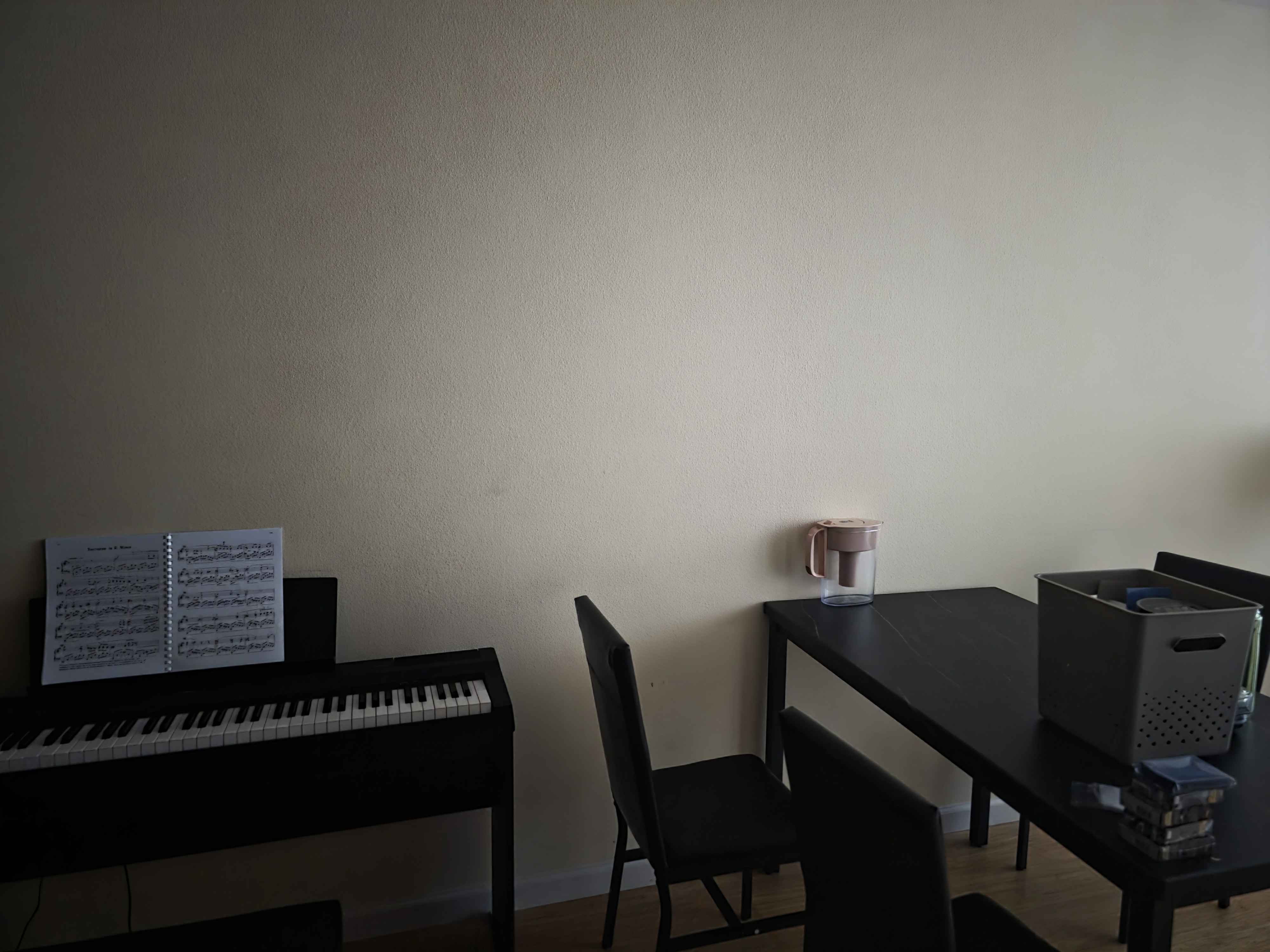
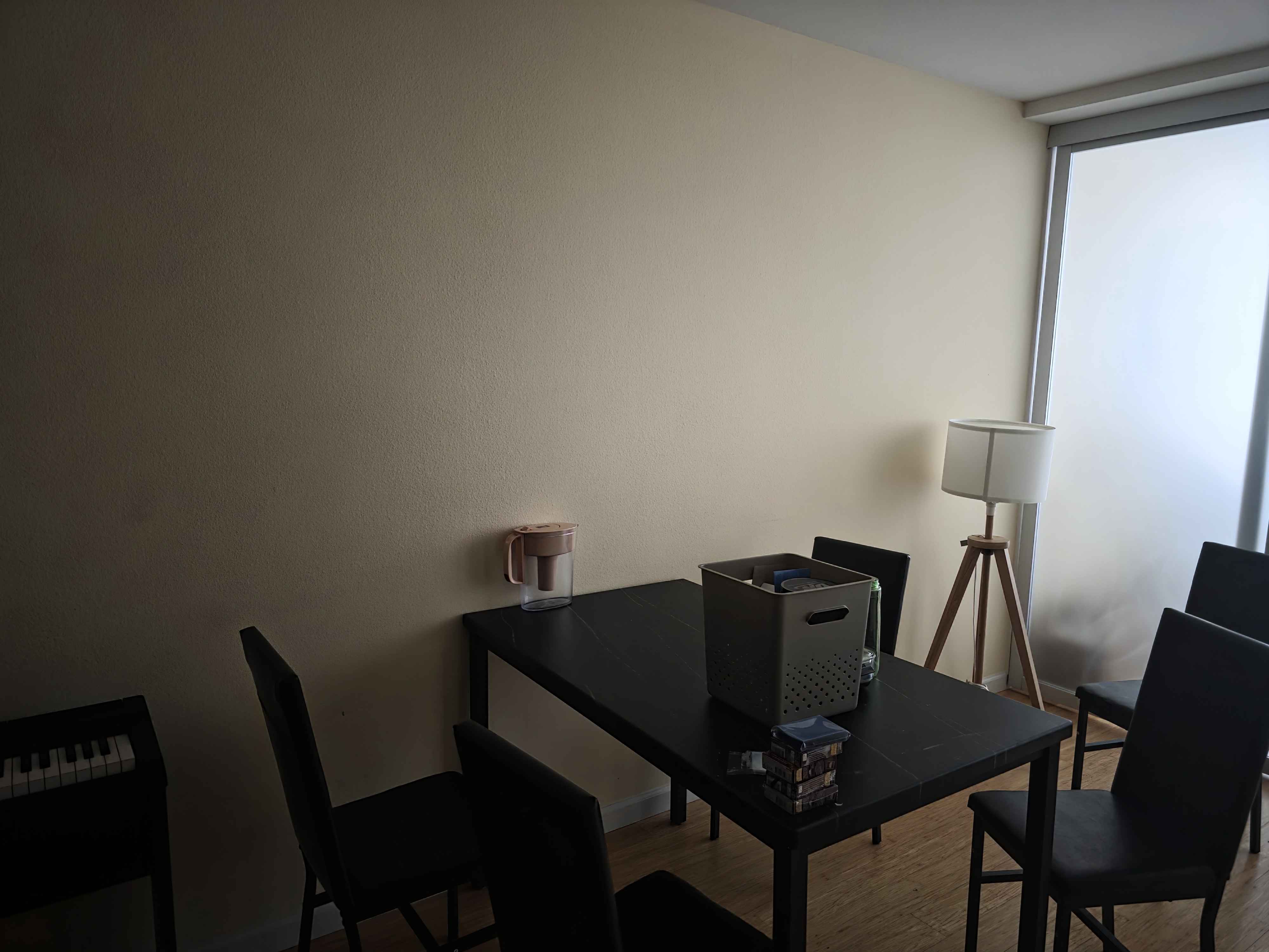
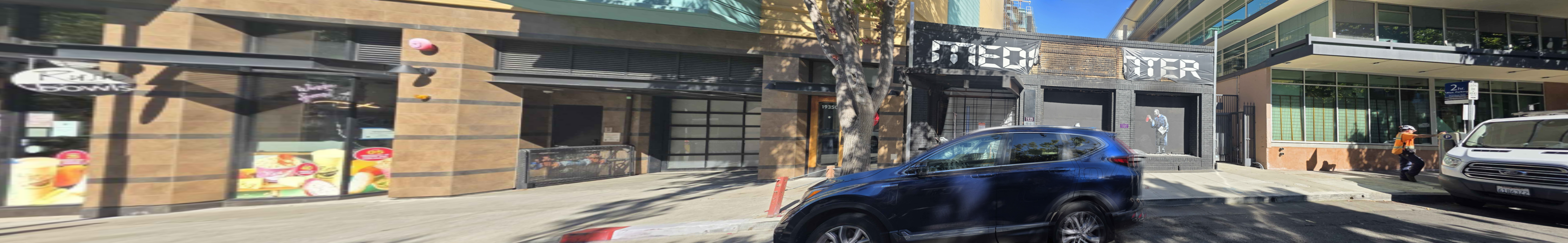
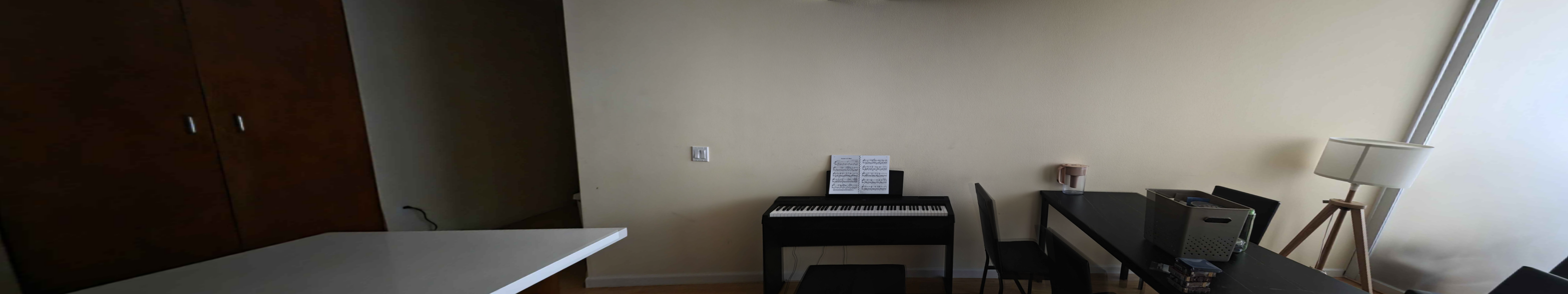
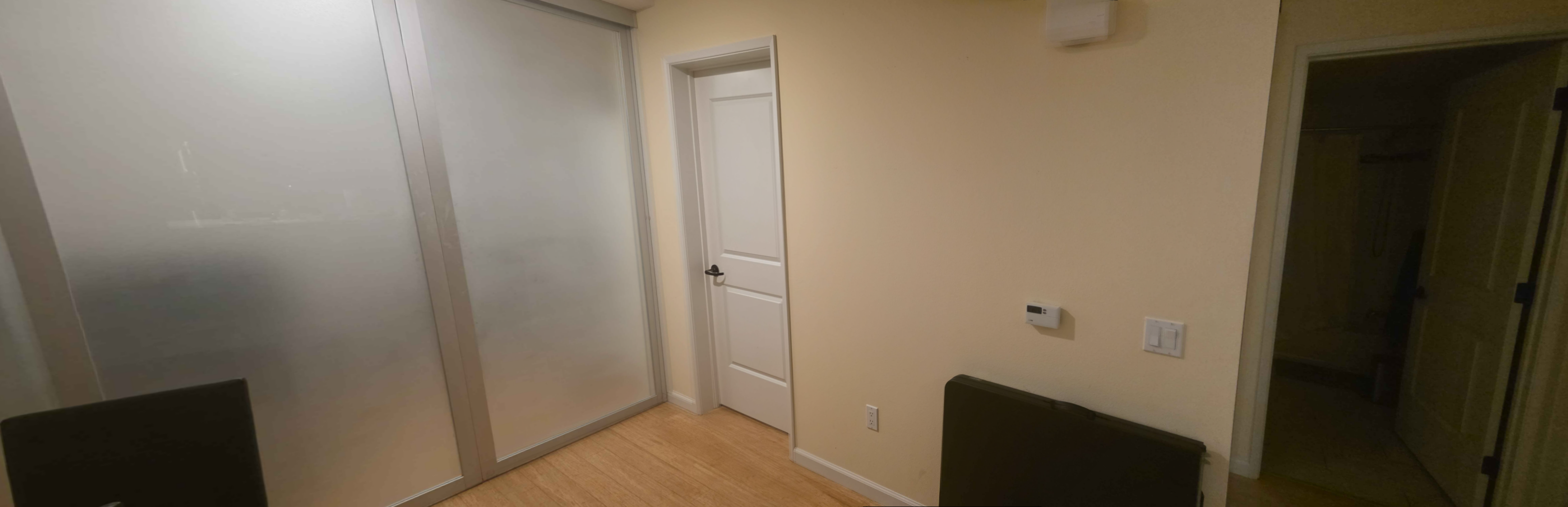
Here are the set of images that I used to calculate the homography and warp and mosaics.

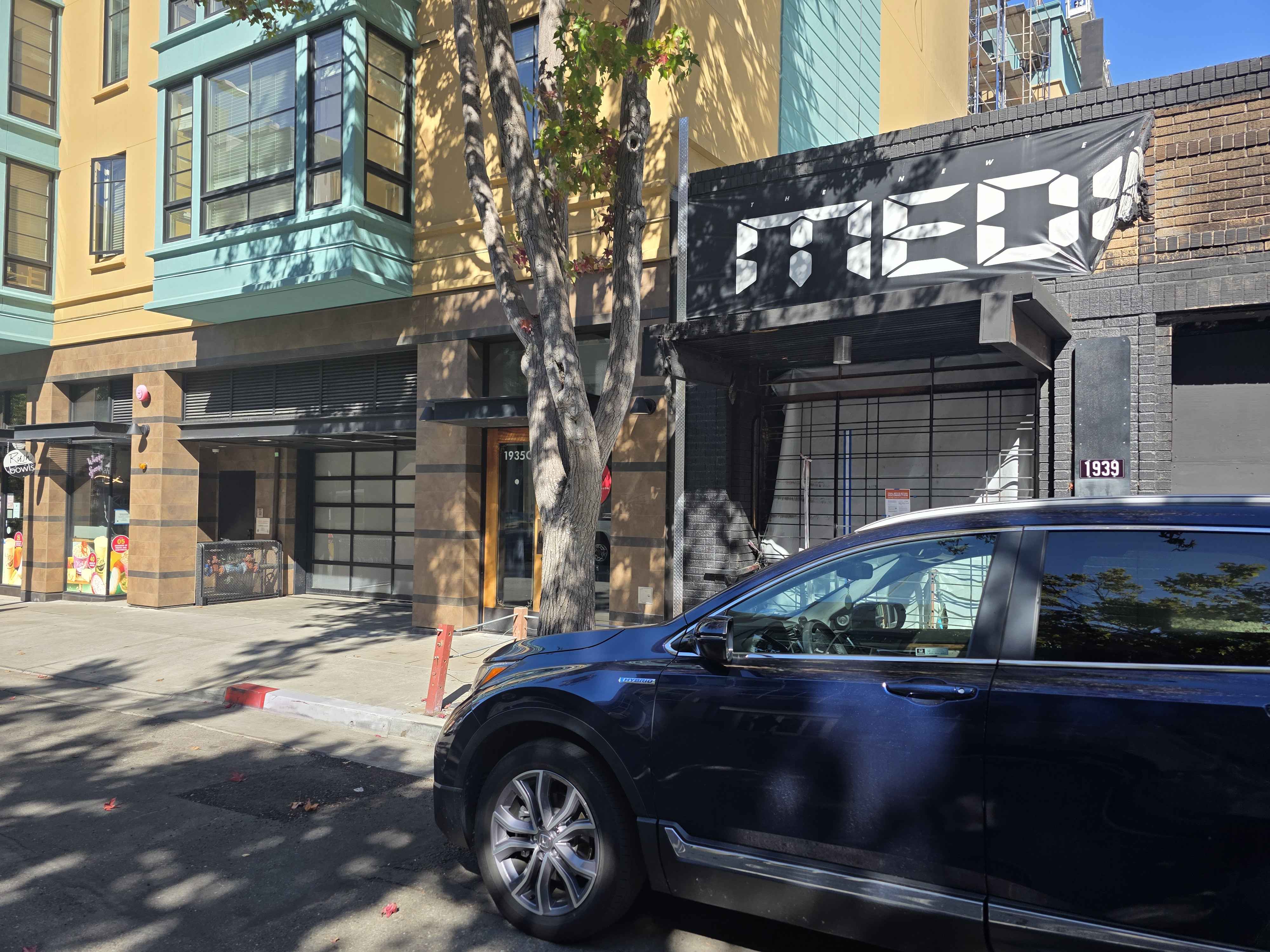
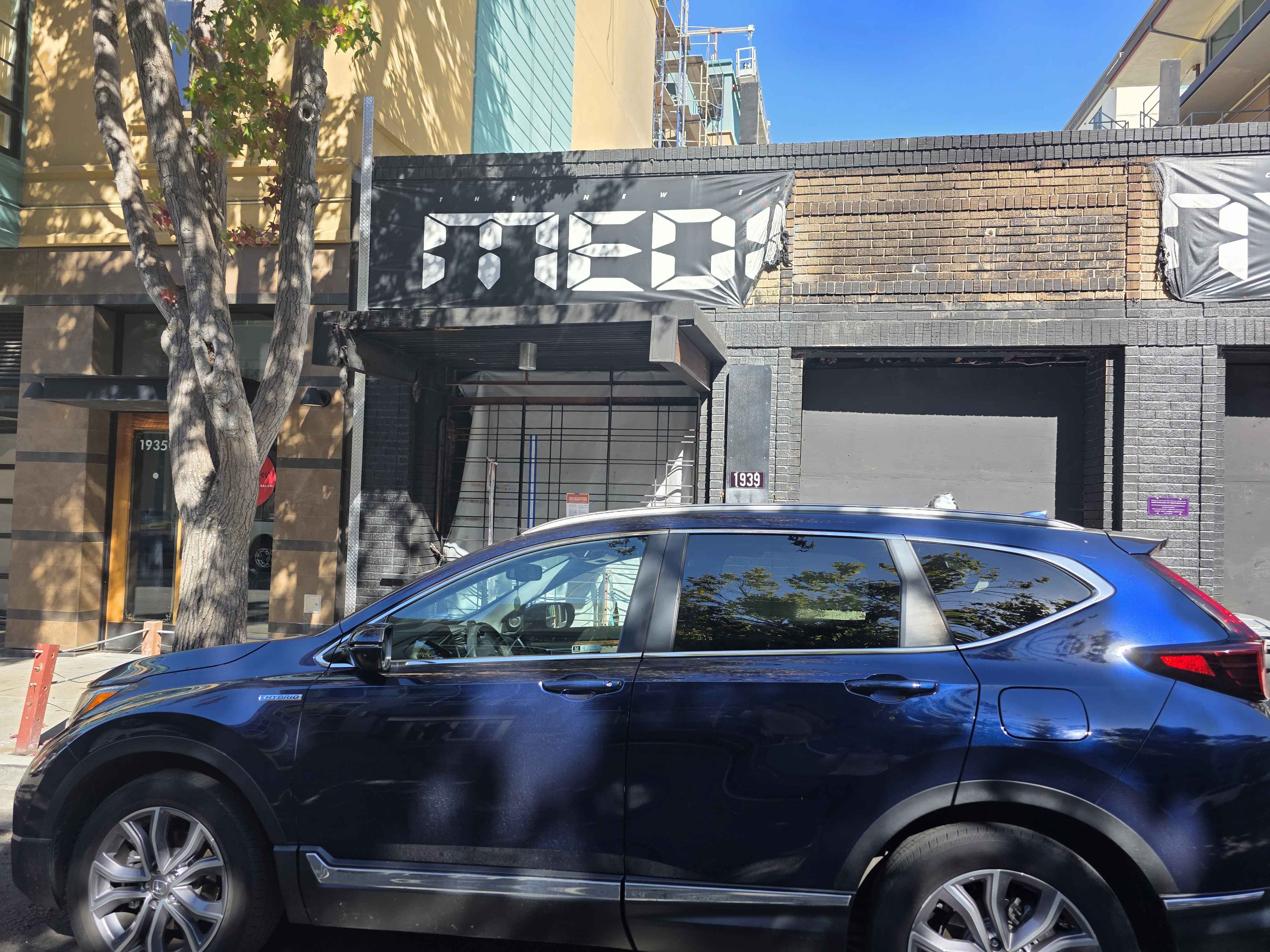
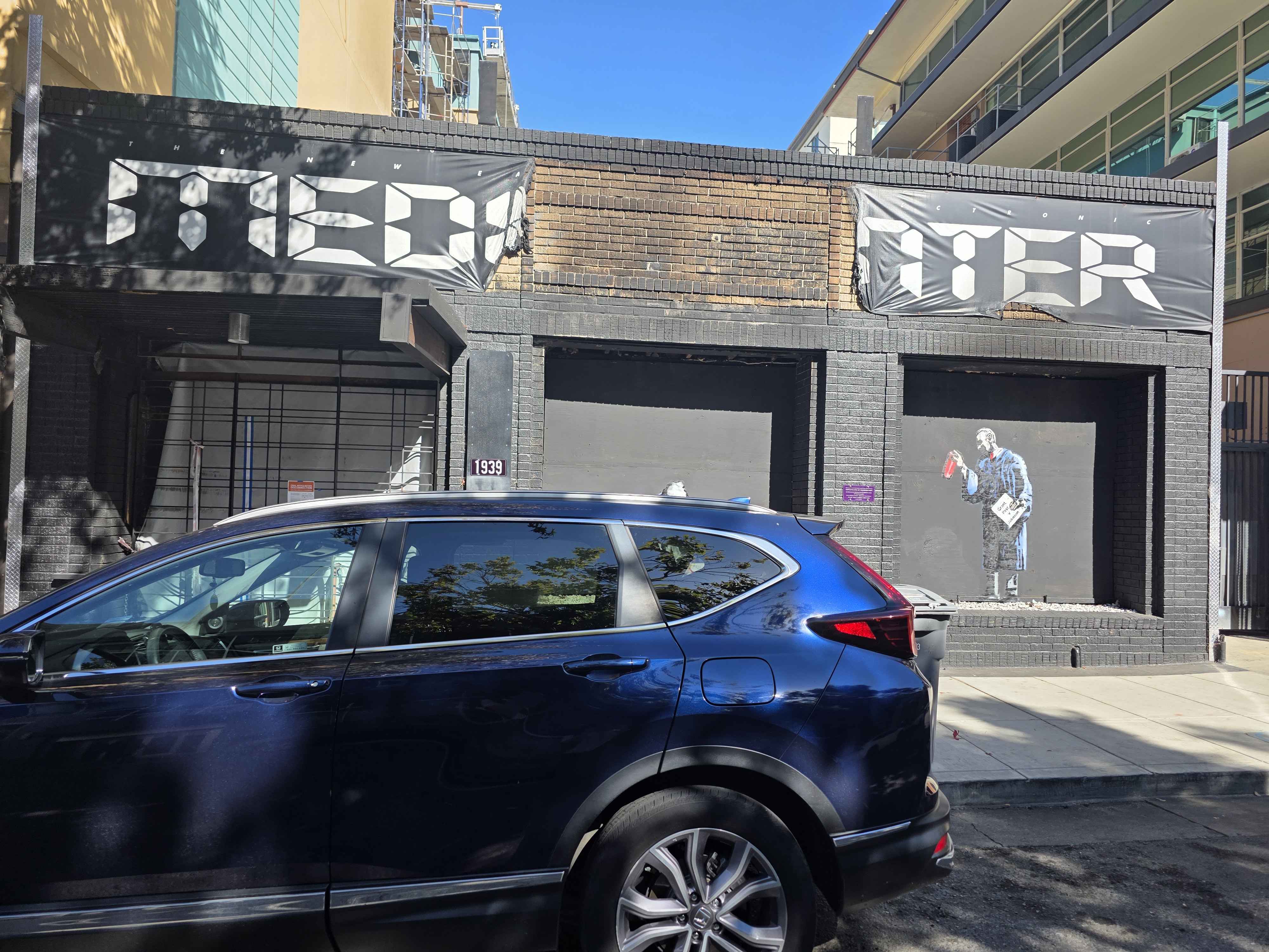
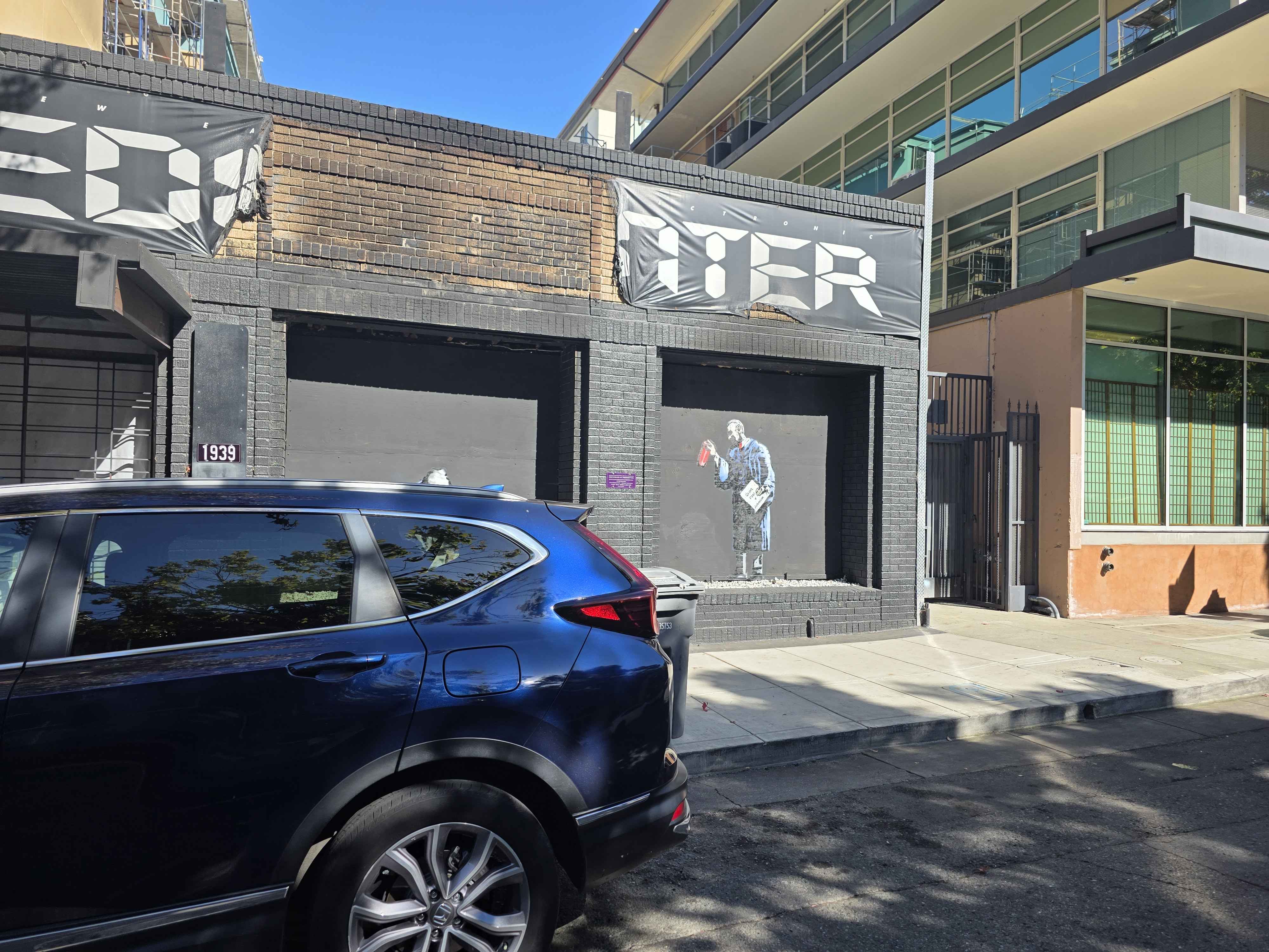
Here is another set of images that I used.

Part A.2

Homography from Point Correspondences System of Equations

Given a point $\mathbf p = [x, y, 1]^\top$ in image 1 and its correspondence $\mathbf p' = [x', y', 1]^\top$ in image 2 (both in homogeneous coordinates), a planar/projective mapping is:

\mathbf p' \sim H\,\mathbf p, \qquad H=\begin{bmatrix} h_{11} & h_{12} & h_{13}\\ h_{21} & h_{22} & h_{23}\\ h_{31} & h_{32} & h_{33} \end{bmatrix}

Writing $\tilde{\mathbf p}' = H\mathbf p = [X', Y', Z']^\top$ and converting back to Euclidean coordinates gives:

x'=\frac{X'}{Z'}=\frac{h_{11}x+h_{12}y+h_{13}}{h_{31}x+h_{32}y+h_{33}},\qquad y'=\frac{Y'}{Z'}=\frac{h_{21}x+h_{22}y+h_{23}}{h_{31}x+h_{32}y+h_{33}}

Clearing denominators yields two linear equations in the entries of H:

\begin{align} x'(h_{31}x+h_{32}y+h_{33}) &= h_{11}x+h_{12}y+h_{13}\\ y'(h_{31}x+h_{32}y+h_{33}) &= h_{21}x+h_{22}y+h_{23} \end{align}

Rearranging each to the left-hand side:

\begin{align} x\,h_{11}+y\,h_{12}+1\cdot h_{13} - x'x\,h_{31} - x'y\,h_{32} - x'\,h_{33} &= 0\\ x\,h_{21}+y\,h_{22}+1\cdot h_{23} - y'x\,h_{31} - y'y\,h_{32} - y'\,h_{33} &= 0 \end{align}

H₃₃ = 1 as per the spec, so solve for the remaining eight unknowns:

\mathbf h_8 = \begin{bmatrix} h_{11}&h_{12}&h_{13}&h_{21}&h_{22}&h_{23}&h_{31}&h_{32} \end{bmatrix}^\top

For one correspondence, this becomes:

\underbrace{\begin{bmatrix} x & y & 1 & 0 & 0 & 0 & -x x' & -y x'\\ 0 & 0 & 0 & x & y & 1 & -x y' & -y y' \end{bmatrix}}_{A_i \in \mathbb R^{2\times 8}} \mathbf h_8 = \underbrace{\begin{bmatrix} x' \\ y' \end{bmatrix}}_{\mathbf b_i}

Stacking all pairs gives the overdetermined system:

A\,\mathbf h_8 = \mathbf b,\qquad A=\begin{bmatrix} A_1\\ \vdots\\ A_n\end{bmatrix}\in\mathbb R^{2n\times 8},\quad \mathbf b=\begin{bmatrix} \mathbf b_1\\ \vdots\\ \mathbf b_n\end{bmatrix}\in\mathbb R^{2n}

Solve in the least-squares sense:

\min_{\mathbf h_8}\;\|A\mathbf h_8-\mathbf b\|_2^2

Then reconstruct:

H = \begin{bmatrix} h_{11} & h_{12} & h_{13}\\ h_{21} & h_{22} & h_{23}\\ h_{31} & h_{32} & 1 \end{bmatrix}

The Results

Here are the two images that I used to calculate homography:

Here are the corresponding points and homography matrix:

Homography Matrix:

H = \begin{bmatrix} 1.5577 & -0.1154 & -1771.93\\ 0.2938 & 1.3431 & -739.49\\ 0.0001 & -0.0000 & 1.0000 \end{bmatrix}

Corresponding Points:

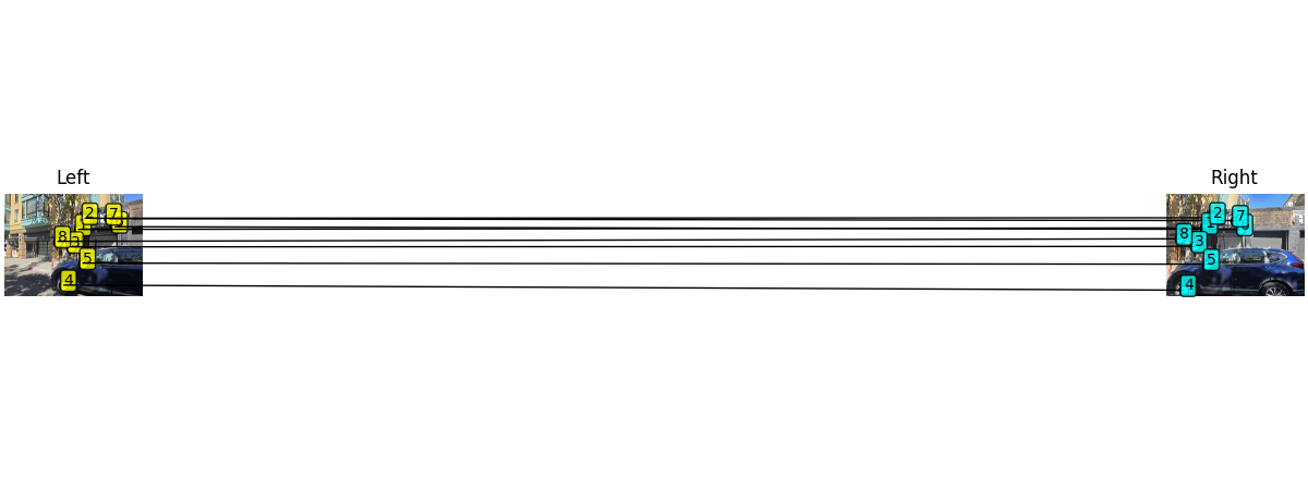
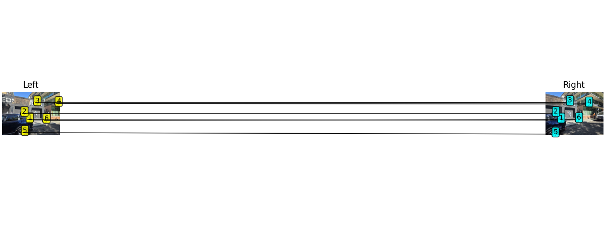
\text{im1\_pts} = \begin{bmatrix} 2145.48 & 1045.54\\ 2345.31 & 719.74\\ 1919.59 & 1553.80\\ 1719.76 & 2665.89\\ 2275.80 & 2027.31\\ 3205.44 & 967.35\\ 3036.02 & 732.77\\ 1545.99 & 1393.07 \end{bmatrix}

\text{im2\_pts} = \begin{bmatrix} 1132.40 & 1002.10\\ 1362.64 & 706.70\\ 832.66 & 1540.77\\ 515.54 & 2813.59\\ 1184.53 & 2057.72\\ 2153.26 & 1045.54\\ 2022.94 & 789.24\\ 389.56 & 1319.22 \end{bmatrix}

The homography matrix H transforms points from image 1 to image 2 coordinates. Each row in the point matrices represents a correspondence: the i-th row of im1_pts corresponds to the i-th row of im2_pts. I think I could have perhaps chosen more accurate points, but oh well. Here are the points visualized:

Here are some additional homographies calculated from different imgaes. Here are the images:

Here are the homography matrices:

H = \begin{bmatrix} 1.2768 & -0.0563 & -1088.52\\ 0.0930 & 1.0826 & -162.86\\ 0.0001 & -0.0000 & 1.0000 \end{bmatrix}

Here are the corresponding points:

\text{im1\_pts} = \begin{bmatrix} 1763.20 & 1931.74\\ 1402.64 & 1501.67\\ 2297.52 & 754.49\\ 3774.51 & 806.62\\ 1433.05 & 2826.62\\ 2931.76 & 1975.18 \end{bmatrix}

\text{im2\_pts} = \begin{bmatrix} 949.95 & 1953.46\\ 589.39 & 1501.67\\ 1566.81 & 737.11\\ 2891.76 & 837.03\\ 563.33 & 2926.53\\ 2192.36 & 1923.05 \end{bmatrix}

And here are the points visualized:

Part A.3

For this part, I decided to warp the second set of images I showed above. Here is the reference image and image to be warped, for reference:

Image to be warped

Reference image

Here are the results of warping the image using bilinear and nearest neighbor interpolation:

Bilinear Interpolation

Nearest Neighbor Interpolation

Here are the results on the first set of images. Here are the images first:

Image to be warped

Reference image

Here are the results:

Bilinear Interpolation

Nearest Neighbor Interpolation

The main difference between bilinear and nearest neighbor interpolation is that bilinear interpolation is smoother and more accurate, but takes more time. As you can see from the nearest neighbor warped images, they kind of look a little off (though you have to look very closely to find aliasing). Since the bilinear images are smoother, they have less aliasing, but they also look a little bit more blurry.

Part A.4

To construct mosaics, I fist compute homographies of each image with the next image. Then, I choose an image as the middle, unwarped image, which is the middle image by default. I first warp all the other images to this reference imgae to determine how big the final output canvas will be. Later on, I added code to scale it down if it was too big because otherwise it would take too much memory and actually crash. But anyway, I then create an additional transformation that transforms everything so that they can properly fit on the canvas (so that the top left of the canvas is 0,0 for all images). This can be multiplied along with the scaling transformation and the homographies to warp each image. Before warping though, I have to first prepare to use alpha blending with arrays to store the alpha values and colors for each pixel. Then, using cosine interpolation, I build the alpha mask for each image using its own coordinates, then finally warp each image along with its alpha mask. I also had to use another mask to set all values to 0 for pixels outside of each image. Then, I finally add everything together and normalize to get the final image. This method of using the alpha mask with interpolation does the feathering, since it makes the edges of the images the weighted averages of the different images based on the alpha values.

Here is the completed mosaic with the set of images from above. I perhaps made a mistake in not using more zoomed in shots, since the camera on my phone is a pretty wide angle with lots of distortion on the sides.

Here is the mosaic with the second set of images. Note that the huge distortion is because I used the middle image as the one to keep unchanged, and the right image is very distorted relative to the other images (wide ish lense plus large angle).

Here is what it looks like when we don't include the last image:

Part B.1

Here is one of the images from above with the Harris corners overlayed. I had to change some of the arguments for the harris function used since my image was so high resolution and it returned too many corners by default.

Here is the result of anms. I used the default arguments for the harris function for this one since it returned more points, allowing for more spread out points for anms. Pretty cool huh.

Part B.2

Here are some of features extracted from the above image. They have been englarged to be actuall visible.

Part B.3

Here are some of the matched features from images 1 and 2. On the top row are the features from image 1 and the second row shows features from image 2. You can see that they look pretty much the same.

Part B.4

Now it is finally time to RANSAC to create auto mosaics. I ran into a lot of problems with this part, especially because the images I used were so large that the program would take forever to run (more than 10 minutes) and would also sometimes crash due to memory usage since the output image is so big. It helped to downscale the images first, and I also changed how we match image pairs. Rather than brute forcing it, I put feature into a KD tree and search for the nearest neighbors by quering the tree, which is usually faster than the linear time search that a normal search would take. Anyway, then we run RANSAC to find the best homography between the two images.

Here are some of the above manually made mosaics from above side by side with the automatically made mosaics.

Manual Mosaic of images 1 to 5

Automatic Mosaic of images 1 to 5

Manual Mosaic of images 6 to 10

Automatic Mosaic of images 6 to 10

As you can see from the results, the mosaics with automatically chosen homogreaphies tend to be much straigher on the sides, and this is because my manually chosen points tend to be slightly off vertically and horizontally, leading to the large warpings. Any additional waprings is probably because I didn't take each photo completely vertically (some are slightly tilted). Here is a final image made with the auto mosaic to fulfill the requirement.

Final mosaic with a new set of images

But what's up with the stupid bowtie shape of all the images? This is mainly just because I use the center image as the reference and warp everything around it. Since each image is fairly distorted to begin with (wide ish angle lense), that means the other images have to be warped a lot more, which just compounds with more images and makes the images on the edge a lot taller. I'm not sure if we are required to fix this, but I tried to do so anyway because I don't want to lose points otherwise. The easiest way to fix it would just be to crop eveyrhting down to remove any blank space. Here are the results of the cropped images.

Mosaic of images 1 to 5 cropped

Mosaic of images 6 to 10 cropped

Mosaic of images 11 to 14 cropped

The other way to fix this would be to warp the images first so that their output shape is properly rectangle, which can also help us end up with consistent final image shapes.